GTEx
N
2022
Last updated: 2023-08-30
Checks: 6 1
Knit directory: lab-notes/
This reproducible R Markdown analysis was created with workflowr (version 1.7.0). The Checks tab describes the reproducibility checks that were applied when the results were created. The Past versions tab lists the development history.
Great! Since the R Markdown file has been committed to the Git repository, you know the exact version of the code that produced these results.
Great job! The global environment was empty. Objects defined in the global environment can affect the analysis in your R Markdown file in unknown ways. For reproduciblity it’s best to always run the code in an empty environment.
The command set.seed(1) was run prior to running the
code in the R Markdown file. Setting a seed ensures that any results
that rely on randomness, e.g. subsampling or permutations, are
reproducible.
Nice! There were no cached chunks for this analysis, so you can be confident that you successfully produced the results during this run.
Great job! Using relative paths to the files within your workflowr project makes it easier to run your code on other machines.
Great! You are using Git for version control. Tracking code development and connecting the code version to the results is critical for reproducibility.
The results in this page were generated with repository version ba8cc1d. See the Past versions tab to see a history of the changes made to the R Markdown and HTML files.
Note that you need to be careful to ensure that all relevant files for
the analysis have been committed to Git prior to generating the results
(you can use wflow_publish or
wflow_git_commit). workflowr only checks the R Markdown
file, but you know if there are other scripts or data files that it
depends on. Below is the status of the Git repository when the results
were generated:
Ignored files:
    Ignored:    analysis/doc_prefix.html
Note that any generated files, e.g. HTML, png, CSS, etc., are not included in this status report because it is ok for generated content to have uncommitted changes.
These are the previous versions of the repository in which changes were
made to the R Markdown (analysis/gtex.Rmd) and HTML
(docs/gtex.html) files. If you’ve configured a remote Git
repository (see ?wflow_git_remote), click on the hyperlinks
in the table below to view the files as they were in that past version.
| File | Version | Author | Date | Message |
|---|---|---|---|---|
| html | d9c3393 | 1onic | 2023-08-28 | Build site. |
| html | d4afa3b | 1onic | 2023-07-12 | Build site. |
| html | 289324b | 1onic | 2023-07-12 | Build site. |
| html | be52451 | 1onic | 2023-07-12 | Build site. |
| html | a73ac21 | 1onic | 2023-06-13 | Build site. |
| html | 41874f0 | 1onic | 2023-06-13 | Build site. |
| html | 75989aa | 1onic | 2023-06-13 | Build site. |
| html | 14b2f73 | 1onic | 2023-06-13 | Build site. |
| html | 6f3f6a4 | 1onic | 2023-05-17 | Build site. |
| html | 5192404 | 1onic | 2023-05-17 | Build site. |
| html | 93a8936 | 1onic | 2023-05-10 | Build site. |
| html | 454b232 | 1onic | 2023-05-10 | Build site. |
| html | 6a1bef0 | 1onic | 2023-05-10 | Build site. |
| html | b8fbbd1 | 1onic | 2023-05-10 | Build site. |
| html | e5648db | 1onic | 2023-05-10 | Build site. |
| html | c0c4bf0 | 1onic | 2023-04-26 | Build site. |
| html | 9fbd5e6 | 1onic | 2023-04-26 | Build site. |
| html | 1478db1 | 1onic | 2023-04-19 | Build site. |
| html | e1b57ff | 1onic | 2023-03-29 | Build site. |
| html | 7288d9c | 1onic | 2023-03-29 | Build site. |
| html | 3aef7a8 | 1onic | 2023-03-29 | Build site. |
| html | 3f796b6 | 1onic | 2023-03-22 | Build site. |
| html | cdae3ea | 1onic | 2023-03-10 | Build site. |
| html | 99420b0 | 1onic | 2023-03-10 | Build site. |
| html | 0f70ffe | 1onic | 2023-03-10 | Build site. |
| Rmd | 889c495 | 1onic | 2023-03-10 | update |
| html | e4922c1 | 1onic | 2023-03-02 | Build site. |
| html | 2d991e9 | 1onic | 2023-03-02 | Build site. |
| html | c350c44 | 1onic | 2023-02-06 | Build site. |
| html | f12e92e | 1onic | 2023-02-06 | Build site. |
| html | 0b2cc20 | 1onic | 2023-02-06 | Build site. |
| html | fdd0022 | 1onic | 2023-02-06 | Build site. |
| html | 21d42f1 | 1onic | 2023-01-27 | Build site. |
| html | e47cac4 | 1onic | 2023-01-27 | Build site. |
| html | bce6cff | 1onic | 2023-01-11 | Build site. |
| html | c51b055 | 1onic | 2023-01-11 | Build site. |
| html | baf3f16 | 1onic | 2023-01-11 | Build site. |
| html | f1c0cc6 | 1onic | 2023-01-11 | Build site. |
| html | cbbb209 | 1onic | 2022-12-09 | Build site. |
| html | fec1e8a | 1onic | 2022-12-09 | Build site. |
| html | 5006f39 | 1onic | 2022-08-04 | Build site. |
| html | a6f860c | 1onic | 2022-08-04 | Build site. |
| html | 57e862a | 1onic | 2022-08-04 | Build site. |
| html | d9c1a09 | 1onic | 2022-08-04 | Build site. |
| html | 8a38159 | 1onic | 2022-08-04 | Build site. |
| html | 12331d2 | 1onic | 2022-08-04 | Build site. |
| html | c814105 | 1onic | 2022-08-04 | Build site. |
| html | c92e0bf | 1onic | 2022-08-03 | Build site. |
| html | 16b143f | 1onic | 2022-07-20 | Build site. |
| html | 3393b21 | 1onic | 2022-07-20 | Build site. |
| html | a0de791 | 1onic | 2022-07-20 | Build site. |
| html | bdf7cc6 | 1onic | 2022-07-20 | Build site. |
| html | 02d90b5 | 1onic | 2022-07-20 | Build site. |
| html | 0c1180e | 1onic | 2022-07-20 | Build site. |
| html | 52e007d | 1onic | 2022-07-20 | Build site. |
| html | 1b61926 | 1onic | 2022-07-20 | Build site. |
| html | fd6de4c | 1onic | 2022-07-20 | Build site. |
| html | 635a240 | 1onic | 2022-07-15 | Build site. |
| html | d13dab9 | 1onic | 2022-07-13 | Build site. |
| html | 695caed | 1onic | 2022-07-13 | Build site. |
| html | ff7c8b1 | 1onic | 2022-07-13 | Build site. |
| html | a8c96b0 | 1onic | 2022-07-07 | Build site. |
| html | b06249e | 1onic | 2022-07-07 | Build site. |
| html | 04de0ae | 1onic | 2022-06-29 | Build site. |
| html | 2da0805 | 1onic | 2022-06-29 | Build site. |
| html | 5eee051 | 1onic | 2022-06-29 | Build site. |
| html | 1516b6d | 1onic | 2022-06-29 | Build site. |
| html | 28a9475 | 1onic | 2022-06-28 | Build site. |
| html | 58646b4 | 1onic | 2022-06-15 | Build site. |
| html | f4b1305 | 1onic | 2022-06-15 | Build site. |
| Rmd | 9432cfd | 1onic | 2022-06-15 | update |
| html | cc4be00 | N | 2022-05-18 | Build site. |
| Rmd | 2ead4a4 | N | 2022-05-18 | update |
| html | 1401122 | N | 2022-05-18 | Build site. |
| Rmd | 6e569ec | N | 2022-05-18 | update |
| html | 557a2a9 | N | 2022-05-18 | Build site. |
| Rmd | 910178f | N | 2022-05-18 | update |
| html | c41d4f9 | N | 2022-05-12 | Build site. |
| html | 1261222 | N | 2022-05-12 | Build site. |
| html | 90df802 | N | 2022-05-11 | Build site. |
| Rmd | 633245f | N | 2022-05-11 | update |
| html | 6e985df | N | 2022-05-11 | Build site. |
| Rmd | 147b522 | N | 2022-05-11 | gtex update |
| html | a844654 | N | 2022-05-11 | Build site. |
| Rmd | 21bcd74 | N | 2022-05-11 | update |
| html | aa46898 | N | 2022-05-11 | Build site. |
| html | d79e35c | N | 2022-05-11 | Build site. |
| html | bfc20a5 | N | 2022-05-04 | Build site. |
| html | ab1c893 | N | 2022-05-04 | Build site. |
| html | af6c895 | N | 2022-05-04 | Build site. |
| html | 001acfd | N | 2022-04-29 | Build site. |
| html | 52bb457 | N | 2022-04-29 | Build site. |
| html | 947de76 | N | 2022-04-29 | Build site. |
| html | ea30a16 | N | 2022-04-29 | Build site. |
| html | 299e079 | N | 2022-04-29 | Build site. |
| html | 30904e4 | N | 2022-04-29 | Build site. |
| html | 3540605 | N | 2022-04-29 | Build site. |
| html | f681be8 | N | 2022-04-29 | Build site. |
| html | a110a99 | N | 2022-04-27 | Build site. |
| html | 3592f27 | N | 2022-04-27 | Build site. |
| html | 37aa3b8 | N | 2022-04-27 | Build site. |
| html | 5bad46b | N | 2022-04-27 | Build site. |
| html | 7edf2ca | N | 2022-04-27 | Build site. |
| html | f05d18b | N | 2022-04-21 | Build site. |
| html | 976ffc2 | N | 2022-04-21 | Build site. |
| html | 8442797 | N | 2022-04-21 | Build site. |
| html | 695da69 | N | 2022-04-21 | Build site. |
| html | 8e47783 | N | 2022-04-21 | Build site. |
| html | 977ea3e | N | 2022-04-21 | Build site. |
| html | b72fe91 | N | 2022-04-21 | Build site. |
| html | edc54ba | N | 2022-04-21 | Build site. |
| html | dd8b725 | N | 2022-04-21 | Build site. |
| html | e2733c6 | N | 2022-04-21 | Build site. |
| html | 32987ea | N | 2022-04-21 | Build site. |
| html | d1c363f | N | 2022-04-21 | Build site. |
| html | 984b514 | N | 2022-04-21 | Build site. |
| html | a1aa819 | N | 2022-04-21 | Build site. |
| html | 725c775 | N | 2022-04-21 | Build site. |
| html | d31a7f8 | N | 2022-04-21 | Build site. |
| html | 47842f8 | N | 2022-04-21 | Build site. |
| html | c997e70 | N | 2022-04-21 | Build site. |
| html | 2f8b4a5 | N | 2022-04-21 | Build site. |
| html | 3012325 | N | 2022-04-21 | Build site. |
| html | 99fa823 | N | 2022-04-21 | Build site. |
| html | 53e5c0a | N | 2022-04-21 | Build site. |
| html | e2c4450 | N | 2022-04-21 | Build site. |
| html | 67323bc | N | 2022-04-21 | Build site. |
| html | 47fc19a | N | 2022-04-21 | Build site. |
| html | 958dea7 | N | 2022-04-21 | Build site. |
| html | a2b7524 | N | 2022-04-21 | Build site. |
| html | 4b231e9 | N | 2022-04-21 | Build site. |
| html | ea6da48 | N | 2022-04-21 | Build site. |
| html | 56c8aba | N | 2022-04-21 | Build site. |
| html | 649b842 | N | 2022-04-21 | Build site. |
| html | 3a63d56 | N | 2022-04-20 | Build site. |
| html | 6d20288 | N | 2022-04-20 | Build site. |
| Rmd | ad3cbc0 | N | 2022-04-20 | update |
| html | fd4742b | N | 2022-04-07 | Build site. |
| Rmd | a51ee7e | N | 2022-04-07 | update |
| html | fa53b92 | N | 2022-04-07 | Build site. |
| Rmd | fe849b3 | N | 2022-04-07 | update |
| html | b472f9a | N | 2022-04-07 | Build site. |
| Rmd | b59a9de | N | 2022-04-07 | update |
| html | 7240cfb | N | 2022-04-07 | Build site. |
| Rmd | aadc9a0 | N | 2022-04-07 | update |
| html | ecf9247 | N | 2022-04-07 | Build site. |
| Rmd | a7eaa51 | N | 2022-04-07 | update |
| html | e865c25 | N | 2022-04-07 | Build site. |
| Rmd | a74efb7 | N | 2022-04-07 | update |
| html | 3f5f68c | N | 2022-04-07 | Build site. |
| Rmd | 34d0db4 | N | 2022-04-07 | update |
| html | dd23b48 | N | 2022-04-07 | Build site. |
| Rmd | 1a6e8a4 | N | 2022-04-07 | update |
| html | dca45ed | N | 2022-04-07 | Build site. |
| Rmd | 9bff3df | N | 2022-04-07 | update |
| html | 2b73c03 | N | 2022-04-07 | Build site. |
| Rmd | 3d528b7 | N | 2022-04-07 | update |
| html | 047c6b5 | N | 2022-04-07 | Build site. |
| Rmd | 92ed7ab | N | 2022-04-07 | update |
| html | b2d88e7 | N | 2022-04-07 | Build site. |
| Rmd | 6d4d99f | N | 2022-04-07 | update |
| html | 32e9594 | N | 2022-04-07 | Build site. |
| html | 65a9a67 | N | 2022-04-07 | Build site. |
| html | 75c5e7a | N | 2022-04-07 | Build site. |
| Rmd | a8a59f1 | N | 2022-04-07 | update |
5/18/2022 Creating a Mappability-Aware GTF Reference
To create a reference GTF for gene level quantification with RNA-SeQC (reference below) that can take into account the alignability of the exon sequence, we will integrate the Mappability or Uniqueness of Reference Genome from ENCODE for the human genome.
In order to do this, there are several necessary steps.
- Our starting file is one of the window-size seperated, BIGWIG,
tracks. For example, the 36mer one: wgEncodeCrgMapabilityAlign36mer
- The file is in BIGWIG format so it must be converted in two possible ways.
- The first way is to import the BIGWIG directly into R as a GRanges
object using RTracklayer,
a UCSC tool meant for dealing with various annotation track formats such
as bigwig, wig, and other formats.
- The second way is to first convert the BIGWIG into WIG by using the executable BigWig2Wig and then convert it to BED using BEDOPS. The result can be parsed by R easily becuase BED is text based.
- The reference file we are modifying is a GTF file, which is a text
based file so it can be parsed by hand OR we can use rtracklayer again
to import it with import.gff2() (GFF2 or GFF version 2 is identical to
GTF).
- The advantage to using rtracklayer again is that we can also export the modified GRanges object containing the imported GTF relatively easily: export(object, path, format = ‘gff2’), which corresponds to exporting as the original GTF format.
- An important consideration is that the bigwig alignability file
contains tracks that are based on the GRCh37/hg19 genome assembly. If
our GTF reference mismatches this, we need to liftover the bigwig/bed to
the right assembly version.
- This can be done very easily and quickly within R or outside of R.
- If we have an GRanges R object we can actually liftover the entire object with just a single line using the liftover R package. This has the advantage of being several times faster than the CMD line version of liftover. The primary downside is that it is EXTREMELY memory expensive. It was found that calling liftover on the alignability file above, to hg38, costs ~61GB of RAM. Make sure to take this into account, and dont use 64GB limit becuase you might run out for further operations.
- The other way is to use the command line version of Liftover on the BED file.
- Chain files for liftover can be found here chain files
Code so far:
hg19_bigwig_mappability = rtracklayer::import('/project/xuanyao/nikita/mappability/wgEncodeCrgMapabilityAlign36mer.bigWig', format = 'BigWig')
hg19_to_hg38_chain = import.chain('/project/xuanyao/nikita/mappability/hg19ToHg38.over.chain')
hg38_mappability_object <- liftOver(hg19_bigwig_mappability, hg19_to_hg38_chain) # GRanges > GRanges operation
reference <- import.gff2('/project/xuanyao/nikita/mappability/gencode.v26.GRCh38.genes.gtf' ) - Overall Strategy for building new reference.
- Tracks contain a seqname or chromosome name, start, stop, and a alignability score. Tracks also vary in length from 1bp to + ~10,000 bp. Histograms of the track lengths suggests that there are many with lengths of 1-5bp.
- Since we are only interested in high alignability tracks we can subset our GRanges object to only contain tracks with scores of 1.
- We need to take into account several other possibilities when it comes to these regions.
- Use GRanges overlapsAny or findOverlaps to query the exon taken from the refernce to the alignability tracks (of score == 1).
- We should loop exon-by-exon within all exons in the reference GTF using foreach/DoParallel to speed up the process.
One main consideration is that multiple tracks can exists in an exon. When querying the mappability file / GRanges object containing tracks we are not guarenteed to recieve a single (or none) track response.
To handle this I consider 4 cases.
- Case #1: Complete overlap.
- In this case the mappability track with a score of 1 covers the entire exon region. This case is considered first becuase it excludes further steps since we can confidently add the exon as-is to our final GTF since the entire exon is fine.
- Case #2: Inside.
- In this case, we have one (or more) tracks with a score of 1 inside the exon region. In order to handle this we can duplicate the exon and assign each duplicate the correct track.
- This case can lead to a specific exon being split into many smaller parts. For example: we can have two regions of length 5bp that are found within the exon and a larger region towards the end of the exon for a total of 3 regions (corresponding to 3 tracks with alignability scores of 1 located within the exon).
- Case #3: Hang left.
- This case is distict becuase the track covers only a part of the exon from the left side, overlapping with the start of the exon.
- We handle this by assigning the new exon region end to the end of the track, while the location for the beginning of the exon remains the same.
- Case #4: Hang right.
- This is the opposite case as above. This time we handle the corrected exon by assigning the start to the start of the track, and the end of the exon remains the same.
The frequency of these cases can be counted, but hasnt been explored yet.
4/13/2022
QC
The GTEx v8 pipeline has two main QC tools.
The first is the traditional picard mark duplicates. This is run directly on the sorted, aligned BAM files.
# mark duplicates (Picard)
docker run --rm -v $path_to_data:/data -t broadinstitute/gtex_rnaseq:V8 \
    /bin/bash -c "/src/run_MarkDuplicates.py \
        /data/star_out/${sample_id}.Aligned.sortedByCoord.out.patched.bam \
        ${sample_id}.Aligned.sortedByCoord.out.patched.md \
        --output_dir /data"
The second is a pass of a tool called RNA-SeQC authored by Francois Aguet. This tool also performs gene-level quantification based on a GTF file passed as an arguement. (Sample IDs are a bit tricky so they are exrtracted with another tool: ‘bamsync’.)
# RNA-SeQC
docker run --rm -v $path_to_data:/data -t broadinstitute/gtex_rnaseq:V8 \
    /bin/bash -c "/src/run_rnaseqc.py \
    ${sample_id}.Aligned.sortedByCoord.out.patched.md.bam \
    ${genes_gtf} \
    ${genome_fasta} \
    ${sample_id} \
    --output_dir /data"
The following output files are generated in the output directory you provide:
+ {sample}.metrics.tsv : A tab-delimited list of (Statistic, Value) pairs of all statistics and metrics recorded.
+ {sample}.exon_reads.gct : A tab-delimited GCT file with (Exon ID, Gene Name, coverage) tuples for all exons which had at least part of one read mapped.
+ {sample}.gene_reads.gct : A tab-delimited GCT file with (Gene ID, Gene Name, coverage) tuples for all genes which had at least one read map to at least one of its exons. This file contains the gene-level read counts used, e.g., for differential expression analyses.
+ {sample}.gene_tpm.gct : A tab-delimited GCT file with (Gene ID, Gene Name, TPM) tuples for all genes reported in the gene_reads.gct file, with expression values in transcript per million (TPM) units. Note: this file is renamed to .gene_rpkm.gct if the --rpkm flag is present.
+ {sample}.fragmentSizes.txt : A list of fragment sizes recorded, if a BED file was provided
+ {sample}.coverage.tsv : A tab-delimited list of (Gene ID, Transcript ID, Mean Coverage, Coverage Std, Coverage CV) tuples for all transcripts encountered in the GTF.
After both of these tools are run the resulting BAM files are filtered based on the following QC criteria (taken from the output of {sample}.metric.tsv above):
- < 10 million mapped reads
- read mapping rate < 0.2
- intergenic mapping rate > 0.3
- base mismatch rate (mismatched bases divided by total aligned bases) > 0.01 for read mate 1 or > 0.02 for read mate 2
- rRNA mapping rate > 0.3.
The result, on the 702 samples downloaded from the Gen3 data archive, was that all passed the QC checks above. Additionally, the supplementary paper also cites that “outlier samples were identified based on expression profile using a correlation-based statistic and sex incompatibility checks” and that “samples from donors with cytogenetic anomalies (see Section 2) were excluded from analyses”.
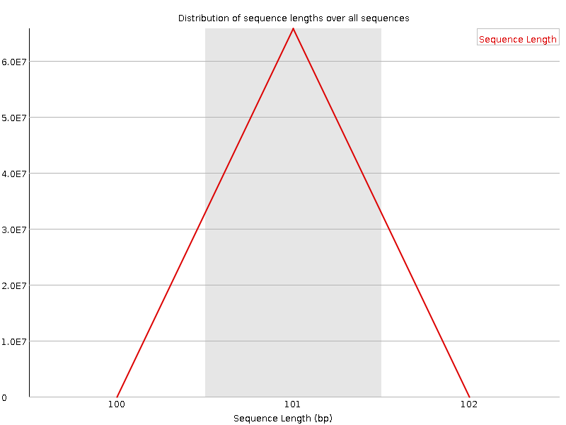
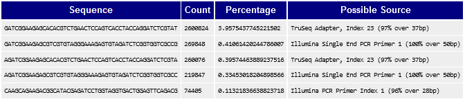
There is 1 sample where the read length is 101 and there also seems to be many adapter sequences.
Read Dist. of Potential Problem Sample O5YV
Overrepresented Sequences IDd by FASTQC in Sample O5YV
4/7/2022
Downloading GTEx v8 Protected Data to HPCs in 2022
Summary: We are downloading the data with the Gen3 client (not Terra bio) specific to a tissue type (or detailed tissue type).
- Get access to data in dbGAP + have a valid server for protected data (ie: HPC Gardner)
The annotation data from the supplementary files contains sample annotations necessary to filter select the files specific to a tissue.
Get annotation data manifest
- Login w/ NIH at https://gen3.theanvil.io/.
- Go the the ‘Downloadable’ tab on the ‘Exploration’ page.
- Select ‘Analysis Supplement’ checkbox to select the 17 supplementary files related to GTEx analysis.
- Click on ‘Download Manifest’
Upload the annotation manifest to HPC system
Download the gen3-client CLI to HPC system
- The latest build for linux can be found here: https://github.com/uc-cdis/cdis-data-client
Generate an API key and upload to HPC system from https://gen3.theanvil.io/identity
Set up the gen3 client CLI with a profile. You will need a profile name (any) and a path to the API key you downloaded in the previous step. You will see a success confirmation.
gen3-client configure --profile=NAME --cred=/path/credentials.json
--apiendpoint=https://gen3.theanvil.io- Remove large/unwanted files from the annotation manifest uploaded in step #2. The ‘Analysis Supplement’ contains both annotation and analysis freezes which are large. This is how it should look afterward:
[
  {
    "object_id": "dg.ANV0/cc511cbe-25de-44a4-873a-9351aa881bef",
    "md5sum": "b3740de6b0550113c48525337d815e0e",
    "file_name": "GTEx_Analysis_2017-06-05_v8_Annotations_SampleAttributesDS.txt",
    "file_size": 15511227
  },
  {
    "object_id": "dg.ANV0/e90fdca7-1d04-4374-bea1-a9c1f4b1fcca",
    "md5sum": "06cabcfe41f504dd2474cb7d73e37014",
    "file_name": "GTEx_Analysis_2017-06-05_v8_Annotations_SubjectPhenotypesDS.txt",
    "file_size": 980021
  },
  {
    "object_id": "dg.ANV0/3e894730-b2d9-4918-9c49-ef700097d25f",
    "md5sum": "2010579d2704a4402ee9b21ba2fdf162",
    "file_name": "GTEx_Analysis_2017-06-05_v8_Annotations_SubjectPhenotypesDD.xlsx",
    "file_size": 34942
  },
  {
    "object_id": "dg.ANV0/3c269f02-76a9-4dde-9b65-bb6a6bb9be06",
    "md5sum": "53c50d3e172c754cd80a24b8093fb229",
    "file_name": "GTEx_Analysis_2017-06-05_v8_Annotations_SampleAttributesDD.xlsx",
    "file_size": 17272
  }
]- Download the annotation data with the following command using the gen3-client CLI + profile + API key + annotation manifest:
/path/gen3-client download-multiple --profile=NAME --manifest=/path/file-manifest-we-will-download.json
--download-path=/path/output_directory
--protocol=s3 --numparallel=5 --skip-completed
Next, we will need to download the main data manifest. This step is generalizable and depends on what data you are looking to download.
- Download data manifest for aligned, RNA-Seq files from https://gen3.theanvil.io/
- For RNA Seq data we select ‘RNA-Seq’ in the ‘Seqeuencing Assay’ subsection of the downloadable data tab. (For WGS data, we would select ‘WGS’ )
- We need to specify the file-type: for our case we want aligned BAM files and their corresponding BAI files. So we select Data Type > ‘Aligned Reads’ and Data Format > ‘BAM’ + ‘BAI’
- Click on ‘Download Manifest’
- Upload the RNA-Seq data manifest to HPC system
For the next step we need to filter the data manifest from the previous step, based on the tissue type or other parameters.
- Filter the data manifest. Strategy: JSON > flatten to data.table > dplyr filter > back to JSON
Example:
library(dplyr)
library(data.table)
library(jsonlite)
# read annotation table downloaded in step #2
anno =  data.table::fread(paste0('/path/GTEx_Analysis_2017-06-05_v8_Annotations_SampleAttributesDS.txt'), stringsAsFactors = F, header = T, sep='\t')

# select the data type and tissue type we want
# assigned a new column: INDV which contains the individual id extracted from the GUID/sample ID.
s1 = anno %>% filter(SMAFRZE == 'RNASEQ', SMTSD == 'Muscle - Skeletal') %>% rowwise() %>% mutate(INDV = strsplit(as.character(SAMPID),"-")[[1]][2])
s2 = anno %>% filter(SMAFRZE == 'WGS') %>% rowwise() %>% mutate(INDV = strsplit(as.character(SAMPID),"-")[[1]][2])

# find RNA-Seq sample guid ids (bonus WGS sample guid ids) which correspond to individuals with both RNA-Seq data AND WGS data (n=706).
common_SAMPID_RNA = s1 %>% filter(INDV %in% intersect(s1$INDV, s2$INDV)) %>% pull(SAMPID)
#common_SAMPID_DNA = s2 %>% filter(INDV %in% intersect(s1$INDV, s2$INDV)) %>% pull(SAMPID)
# the n=706 comes from length(intersect(s1$INDV, s2$INDV))

# read file manifest downloaded in step #6
manifest = fromJSON('/path/file-manifest.json')
try = as.data.table(manifest) %>% rowwise() %>% mutate(SAMPID = strsplit(file_name, '[.]')[[1]][1]) %>% filter(SAMPID %in% common_SAMPID_RNA) %>% select(-SAMPID)
subset_manifest = toJSON(try, dataframe = 'rows', pretty = TRUE)
write(subset_manifest, "/path/file-manifest-we-will-download.json")- Next we will download the data using the filtered manifest:
/path/gen3-client download-multiple --profile=NAME --manifest=/path/file-manifest-we-will-download.json
--download-path=/path/output_directory
--protocol=s3 --skip-completed
Notice the use of –skip-completed in order to resume paused downloads and –numparallel
Update the gen3 tool might have a bug
As of 3/~6/2023 I found that using the –numparallel=5 flag results in 404 and fail. I am unsure what is causing this so please dont use it atm.
- Repeat for other data selections (other tissues, WGS CRAM data, etc.) by modifying the filtering performed above.
Example for Esophagus - Muscularis:
s1 = anno %>% filter(SMAFRZE == 'RNASEQ', SMTSD == 'Esophagus - Muscularis') %>% rowwise() %>% mutate(INDV = strsplit(as.character(SAMPID),"-")[[1]][2])