sceptre
N
2022
Last updated: 2023-09-20
Checks: 6 1
Knit directory: lab-notes/
This reproducible R Markdown analysis was created with workflowr (version 1.7.0). The Checks tab describes the reproducibility checks that were applied when the results were created. The Past versions tab lists the development history.
Great! Since the R Markdown file has been committed to the Git repository, you know the exact version of the code that produced these results.
Great job! The global environment was empty. Objects defined in the global environment can affect the analysis in your R Markdown file in unknown ways. For reproduciblity it’s best to always run the code in an empty environment.
The command set.seed(1) was run prior to running the
code in the R Markdown file. Setting a seed ensures that any results
that rely on randomness, e.g. subsampling or permutations, are
reproducible.
Nice! There were no cached chunks for this analysis, so you can be confident that you successfully produced the results during this run.
Great job! Using relative paths to the files within your workflowr project makes it easier to run your code on other machines.
Great! You are using Git for version control. Tracking code development and connecting the code version to the results is critical for reproducibility.
The results in this page were generated with repository version 2d1cbd9. See the Past versions tab to see a history of the changes made to the R Markdown and HTML files.
Note that you need to be careful to ensure that all relevant files for
the analysis have been committed to Git prior to generating the results
(you can use wflow_publish or
wflow_git_commit). workflowr only checks the R Markdown
file, but you know if there are other scripts or data files that it
depends on. Below is the status of the Git repository when the results
were generated:
Ignored files:
    Ignored:    analysis/doc_prefix.html
Note that any generated files, e.g. HTML, png, CSS, etc., are not included in this status report because it is ok for generated content to have uncommitted changes.
These are the previous versions of the repository in which changes were
made to the R Markdown (analysis/sceptre.Rmd) and HTML
(docs/sceptre.html) files. If you’ve configured a remote
Git repository (see ?wflow_git_remote), click on the
hyperlinks in the table below to view the files as they were in that
past version.
| File | Version | Author | Date | Message |
|---|---|---|---|---|
| Rmd | 2d1cbd9 | 1onic | 2023-09-20 | update |
| html | 5313f6e | 1onic | 2023-09-19 | Build site. |
| html | 56c1b96 | 1onic | 2023-09-19 | Build site. |
| Rmd | a44a325 | 1onic | 2023-09-19 | update |
| html | 039565f | 1onic | 2023-09-19 | Build site. |
| Rmd | 9de327d | 1onic | 2023-09-19 | update |
| html | bde3a61 | 1onic | 2023-09-19 | Build site. |
| Rmd | 639c954 | 1onic | 2023-09-19 | update |
| html | b26555a | 1onic | 2023-09-18 | Build site. |
| Rmd | 86b383c | 1onic | 2023-09-18 | update |
| html | 6a65859 | 1onic | 2023-09-18 | Build site. |
| Rmd | d99966c | 1onic | 2023-09-18 | update |
| html | 6ce0511 | 1onic | 2023-09-18 | Build site. |
| Rmd | 21b2081 | 1onic | 2023-09-18 | update |
| html | 51764ad | 1onic | 2023-09-18 | Build site. |
| Rmd | f72b8f5 | 1onic | 2023-09-18 | update |
| html | 5df5417 | 1onic | 2023-09-11 | Build site. |
| Rmd | 3fc87b6 | 1onic | 2023-09-11 | update |
| html | 9286368 | 1onic | 2023-09-06 | Build site. |
| Rmd | 93764d6 | 1onic | 2023-09-06 | update |
| html | f0b8541 | 1onic | 2023-09-05 | Build site. |
| html | b499a62 | 1onic | 2023-08-30 | Build site. |
| html | f760d8b | 1onic | 2023-08-30 | Build site. |
| html | 9cd8470 | 1onic | 2023-08-30 | Build site. |
| Rmd | deb2992 | 1onic | 2023-08-30 | update |
| html | d9c3393 | 1onic | 2023-08-28 | Build site. |
| Rmd | e203ada | 1onic | 2023-08-28 | update |
| html | d4afa3b | 1onic | 2023-07-12 | Build site. |
| Rmd | 8a6dbfa | 1onic | 2023-07-12 | update |
| html | 289324b | 1onic | 2023-07-12 | Build site. |
| Rmd | 73fe9d7 | 1onic | 2023-07-12 | update |
| html | be52451 | 1onic | 2023-07-12 | Build site. |
| Rmd | 248a74d | 1onic | 2023-07-12 | update |
| html | a73ac21 | 1onic | 2023-06-13 | Build site. |
| Rmd | 27818c3 | 1onic | 2023-06-13 | update |
| html | 41874f0 | 1onic | 2023-06-13 | Build site. |
| Rmd | b66bbb5 | 1onic | 2023-06-13 | update |
| html | 6f3f6a4 | 1onic | 2023-05-17 | Build site. |
| Rmd | 135e88f | 1onic | 2023-05-17 | update |
| html | 5192404 | 1onic | 2023-05-17 | Build site. |
| Rmd | d4ecae8 | 1onic | 2023-05-17 | update |
| html | 93a8936 | 1onic | 2023-05-10 | Build site. |
| Rmd | e58e200 | 1onic | 2023-05-10 | update |
| html | 454b232 | 1onic | 2023-05-10 | Build site. |
| Rmd | cfedb2b | 1onic | 2023-05-10 | update |
| html | 6a1bef0 | 1onic | 2023-05-10 | Build site. |
| Rmd | 6e6664c | 1onic | 2023-05-10 | update |
| html | b8fbbd1 | 1onic | 2023-05-10 | Build site. |
| Rmd | 54b4de8 | 1onic | 2023-05-10 | update |
| html | e5648db | 1onic | 2023-05-10 | Build site. |
| Rmd | 273d6ef | 1onic | 2023-05-10 | update |
| html | c0c4bf0 | 1onic | 2023-04-26 | Build site. |
| Rmd | 2dba149 | 1onic | 2023-04-26 | update |
| html | 9fbd5e6 | 1onic | 2023-04-26 | Build site. |
| Rmd | 58bb0a1 | 1onic | 2023-04-26 | update |
| html | 1478db1 | 1onic | 2023-04-19 | Build site. |
| Rmd | 7345dbd | 1onic | 2023-04-19 | update |
| html | 13ace72 | 1onic | 2023-03-29 | Build site. |
| html | 9b3a894 | 1onic | 2023-03-29 | Build site. |
| Rmd | 126bbf7 | 1onic | 2023-03-29 | update |
| html | e1b57ff | 1onic | 2023-03-29 | Build site. |
| Rmd | 5e606bd | 1onic | 2023-03-29 | update |
| html | 7288d9c | 1onic | 2023-03-29 | Build site. |
| Rmd | f81ed86 | 1onic | 2023-03-29 | update |
| html | 3aef7a8 | 1onic | 2023-03-29 | Build site. |
| Rmd | d9310d1 | 1onic | 2023-03-29 | update |
| html | 3f796b6 | 1onic | 2023-03-22 | Build site. |
| html | d9de43c | 1onic | 2023-03-22 | Build site. |
| Rmd | d6f2632 | 1onic | 2023-03-22 | update |
| html | 730a8bd | 1onic | 2023-03-22 | Build site. |
| Rmd | 081f8b1 | 1onic | 2023-03-22 | update |
| html | e7e33e4 | 1onic | 2023-03-22 | Build site. |
| Rmd | 06566be | 1onic | 2023-03-22 | update |
| html | a5a613b | 1onic | 2023-03-22 | Build site. |
| Rmd | 290efcf | 1onic | 2023-03-22 | update |
| html | cdae3ea | 1onic | 2023-03-10 | Build site. |
| html | 99420b0 | 1onic | 2023-03-10 | Build site. |
| Rmd | 0b86434 | 1onic | 2023-03-10 | update |
| html | 0f70ffe | 1onic | 2023-03-10 | Build site. |
| Rmd | 889c495 | 1onic | 2023-03-10 | update |
| html | e4922c1 | 1onic | 2023-03-02 | Build site. |
| Rmd | 93b9af8 | 1onic | 2023-03-02 | update |
| html | 2d991e9 | 1onic | 2023-03-02 | Build site. |
| Rmd | 06d4b8d | 1onic | 2023-03-02 | update |
| html | 3971f7d | 1onic | 2023-02-15 | Build site. |
| Rmd | 07b5e06 | 1onic | 2023-02-15 | update |
| html | c60273d | 1onic | 2023-02-15 | Build site. |
| Rmd | ba82814 | 1onic | 2023-02-15 | update |
| html | 1d473f7 | 1onic | 2023-02-08 | Build site. |
| Rmd | b9945b4 | 1onic | 2023-02-08 | update |
| html | c350c44 | 1onic | 2023-02-06 | Build site. |
| html | f12e92e | 1onic | 2023-02-06 | Build site. |
| html | 0b2cc20 | 1onic | 2023-02-06 | Build site. |
| html | fdd0022 | 1onic | 2023-02-06 | Build site. |
| Rmd | e24db96 | 1onic | 2023-02-06 | update |
| html | 21d42f1 | 1onic | 2023-01-27 | Build site. |
| html | e47cac4 | 1onic | 2023-01-27 | Build site. |
| Rmd | cd608b0 | 1onic | 2023-01-27 | update |
| html | bce6cff | 1onic | 2023-01-11 | Build site. |
| html | c51b055 | 1onic | 2023-01-11 | Build site. |
| html | baf3f16 | 1onic | 2023-01-11 | Build site. |
| html | f1c0cc6 | 1onic | 2023-01-11 | Build site. |
| Rmd | 40c30e4 | 1onic | 2023-01-11 | update |
| html | 56f1718 | 1onic | 2022-12-14 | Build site. |
| html | e99aeb1 | 1onic | 2022-12-14 | Build site. |
| Rmd | a7161f1 | 1onic | 2022-12-14 | update |
| html | 4913d20 | 1onic | 2022-12-14 | Build site. |
| Rmd | ad1f078 | 1onic | 2022-12-14 | update |
| html | 9fde784 | 1onic | 2022-12-09 | Build site. |
| Rmd | 0a8dde0 | 1onic | 2022-12-09 | update |
| html | 976ccd0 | 1onic | 2022-12-09 | Build site. |
| Rmd | fc4e55c | 1onic | 2022-12-09 | update |
| html | b40a0db | 1onic | 2022-12-09 | Build site. |
| Rmd | 716574f | 1onic | 2022-12-09 | fix plots |
| html | 0b07039 | 1onic | 2022-12-09 | Build site. |
| Rmd | e4c68ad | 1onic | 2022-12-09 | update |
| html | bef0821 | 1onic | 2022-12-09 | Build site. |
| Rmd | 47f4485 | 1onic | 2022-12-09 | update |
| html | cbbb209 | 1onic | 2022-12-09 | Build site. |
| Rmd | 82103da | 1onic | 2022-12-09 | update |
| html | fec1e8a | 1onic | 2022-12-09 | Build site. |
| html | 2be3983 | 1onic | 2022-12-09 | Build site. |
| Rmd | 80f2ffc | 1onic | 2022-12-09 | update |
| html | 6885f3d | 1onic | 2022-10-05 | Build site. |
| Rmd | 39105a4 | 1onic | 2022-10-05 | update |
| html | d3d078e | 1onic | 2022-10-05 | Build site. |
| html | 519a799 | 1onic | 2022-10-05 | Build site. |
| Rmd | d2f2b02 | 1onic | 2022-10-05 | update |
| html | e131c98 | 1onic | 2022-10-04 | Build site. |
| Rmd | 82a40ca | 1onic | 2022-10-04 | update |
| html | e644b7c | 1onic | 2022-10-04 | Build site. |
| Rmd | 7d0a2fe | 1onic | 2022-10-04 | update |
| html | c95047e | 1onic | 2022-10-04 | Build site. |
| Rmd | a382b31 | 1onic | 2022-10-04 | update |
| html | 2387785 | 1onic | 2022-09-21 | Build site. |
| Rmd | 8a86ec9 | 1onic | 2022-09-21 | update |
| html | db3db83 | 1onic | 2022-09-07 | Build site. |
| Rmd | 28cf9c9 | 1onic | 2022-09-07 | update |
| html | 97513f7 | 1onic | 2022-08-30 | Build site. |
| Rmd | df953d6 | 1onic | 2022-08-30 | update |
| html | f7c986f | 1onic | 2022-08-30 | Build site. |
| Rmd | d2013cc | 1onic | 2022-08-30 | update |
| html | 05b39d9 | 1onic | 2022-08-30 | Build site. |
| Rmd | 9047831 | 1onic | 2022-08-30 | update |
| html | 4799da1 | 1onic | 2022-08-30 | Build site. |
| Rmd | 9cc9271 | 1onic | 2022-08-30 | update |
| html | 048a513 | 1onic | 2022-08-30 | Build site. |
| Rmd | 62bdf7e | 1onic | 2022-08-30 | update |
| html | 237f562 | 1onic | 2022-08-30 | Build site. |
| Rmd | 726571f | 1onic | 2022-08-30 | update |
| html | 69a4646 | 1onic | 2022-08-26 | Build site. |
| Rmd | 39b8f0d | 1onic | 2022-08-26 | update |
| html | 5aa7dc2 | 1onic | 2022-08-24 | Build site. |
| Rmd | 1f58a0c | 1onic | 2022-08-24 | update |
| html | 9cf39ab | 1onic | 2022-08-24 | Build site. |
| Rmd | 2aea1e2 | 1onic | 2022-08-24 | update |
| html | 00096ee | 1onic | 2022-08-24 | Build site. |
| Rmd | 1c5014c | 1onic | 2022-08-24 | update |
| html | 375d206 | 1onic | 2022-08-24 | Build site. |
| Rmd | e620871 | 1onic | 2022-08-24 | update |
| html | f52ad4d | 1onic | 2022-08-24 | Build site. |
| Rmd | 30aceb3 | 1onic | 2022-08-24 | update |
| html | 598570e | 1onic | 2022-08-24 | Build site. |
| Rmd | 9a584c1 | 1onic | 2022-08-24 | update |
| html | b4756c4 | 1onic | 2022-08-24 | Build site. |
| Rmd | fbab5cb | 1onic | 2022-08-24 | update |
| html | a55752e | 1onic | 2022-08-24 | Build site. |
| Rmd | da54c09 | 1onic | 2022-08-24 | update |
| html | c97e2d8 | 1onic | 2022-08-24 | Build site. |
| Rmd | d5b953e | 1onic | 2022-08-24 | update |
| html | cece443 | 1onic | 2022-08-10 | Build site. |
| Rmd | f3579f6 | 1onic | 2022-08-10 | MORE PLOTS |
| html | 9955d67 | 1onic | 2022-08-10 | Build site. |
| Rmd | 59aa61b | 1onic | 2022-08-10 | update |
| html | 617a397 | 1onic | 2022-08-10 | Build site. |
| Rmd | 3a438e1 | 1onic | 2022-08-10 | update |
| html | 5208fa3 | 1onic | 2022-08-10 | Build site. |
| Rmd | 6976d77 | 1onic | 2022-08-10 | update |
| html | 7a4197e | 1onic | 2022-08-10 | Build site. |
| Rmd | 9c89a1b | 1onic | 2022-08-10 | update |
| html | bd41509 | 1onic | 2022-08-10 | Build site. |
| Rmd | 1465957 | 1onic | 2022-08-10 | update |
| html | 32d7f10 | 1onic | 2022-08-04 | Build site. |
| Rmd | 8a49a6f | 1onic | 2022-08-04 | update |
| html | 5006f39 | 1onic | 2022-08-04 | Build site. |
| Rmd | e56770a | 1onic | 2022-08-04 | update |
| html | a6f860c | 1onic | 2022-08-04 | Build site. |
| Rmd | fac1ac4 | 1onic | 2022-08-04 | update |
| html | 57e862a | 1onic | 2022-08-04 | Build site. |
| Rmd | 8c00df6 | 1onic | 2022-08-04 | update |
| html | d9c1a09 | 1onic | 2022-08-04 | Build site. |
| Rmd | c4cdc99 | 1onic | 2022-08-04 | update |
| html | 8a38159 | 1onic | 2022-08-04 | Build site. |
| Rmd | e2d078b | 1onic | 2022-08-04 | update |
| html | 12331d2 | 1onic | 2022-08-04 | Build site. |
| Rmd | 2504faa | 1onic | 2022-08-04 | update |
| Rmd | f9e1827 | 1onic | 2022-08-04 | grna comparison |
| html | c814105 | 1onic | 2022-08-04 | Build site. |
| Rmd | 15536d1 | 1onic | 2022-08-04 | update |
| html | c92e0bf | 1onic | 2022-08-03 | Build site. |
| Rmd | 7e88c52 | 1onic | 2022-08-03 | many plots today |
| html | 16b143f | 1onic | 2022-07-20 | Build site. |
| html | 3393b21 | 1onic | 2022-07-20 | Build site. |
| html | a0de791 | 1onic | 2022-07-20 | Build site. |
| html | bdf7cc6 | 1onic | 2022-07-20 | Build site. |
| html | 02d90b5 | 1onic | 2022-07-20 | Build site. |
| html | 0c1180e | 1onic | 2022-07-20 | Build site. |
| html | 52e007d | 1onic | 2022-07-20 | Build site. |
| html | 1b61926 | 1onic | 2022-07-20 | Build site. |
| html | fd6de4c | 1onic | 2022-07-20 | Build site. |
| html | 635a240 | 1onic | 2022-07-15 | Build site. |
| Rmd | 43b30a7 | 1onic | 2022-07-15 | update |
| html | d13dab9 | 1onic | 2022-07-13 | Build site. |
| Rmd | 9d20f03 | 1onic | 2022-07-13 | update |
| html | 695caed | 1onic | 2022-07-13 | Build site. |
| Rmd | 4f3ce77 | 1onic | 2022-07-13 | update |
| html | ff7c8b1 | 1onic | 2022-07-13 | Build site. |
| Rmd | 439a8b1 | 1onic | 2022-07-13 | geo morris qc |
| html | a8c96b0 | 1onic | 2022-07-07 | Build site. |
| html | b06249e | 1onic | 2022-07-07 | Build site. |
| Rmd | 317351e | 1onic | 2022-07-07 | plots and update |
| html | 04de0ae | 1onic | 2022-06-29 | Build site. |
| Rmd | 21ab34f | 1onic | 2022-06-29 | update |
| html | 2da0805 | 1onic | 2022-06-29 | Build site. |
| Rmd | 3ddb896 | 1onic | 2022-06-29 | update |
| html | 5eee051 | 1onic | 2022-06-29 | Build site. |
| Rmd | ba5d409 | 1onic | 2022-06-29 | update |
| html | 1516b6d | 1onic | 2022-06-29 | Build site. |
| Rmd | 8b0a3fb | 1onic | 2022-06-29 | update |
| html | 28a9475 | 1onic | 2022-06-28 | Build site. |
| Rmd | c6f8019 | 1onic | 2022-06-28 | update |
| html | 58646b4 | 1onic | 2022-06-15 | Build site. |
| Rmd | ead2122 | 1onic | 2022-06-15 | update |
| html | f4b1305 | 1onic | 2022-06-15 | Build site. |
| Rmd | 9432cfd | 1onic | 2022-06-15 | update |
| html | cc4be00 | N | 2022-05-18 | Build site. |
| html | 1401122 | N | 2022-05-18 | Build site. |
| html | 557a2a9 | N | 2022-05-18 | Build site. |
| Rmd | 910178f | N | 2022-05-18 | update |
| html | c41d4f9 | N | 2022-05-12 | Build site. |
| Rmd | 916fafa | N | 2022-05-12 | update |
| html | 1261222 | N | 2022-05-12 | Build site. |
| Rmd | 2fa70a3 | N | 2022-05-12 | update |
| html | 90df802 | N | 2022-05-11 | Build site. |
| html | 6e985df | N | 2022-05-11 | Build site. |
| html | a844654 | N | 2022-05-11 | Build site. |
| html | aa46898 | N | 2022-05-11 | Build site. |
| Rmd | 168f3a4 | N | 2022-05-11 | update |
| Rmd | 6170e7a | N | 2022-05-11 | fix plots |
| html | d79e35c | N | 2022-05-11 | Build site. |
| Rmd | 8987b99 | N | 2022-05-11 | update |
| html | bfc20a5 | N | 2022-05-04 | Build site. |
| Rmd | 06a6d40 | N | 2022-05-04 | update |
| html | ab1c893 | N | 2022-05-04 | Build site. |
| Rmd | 9791d29 | N | 2022-05-04 | update |
| html | af6c895 | N | 2022-05-04 | Build site. |
| Rmd | 884eb8e | N | 2022-05-04 | update |
| html | 001acfd | N | 2022-04-29 | Build site. |
| Rmd | 3915adc | N | 2022-04-29 | update |
| html | 52bb457 | N | 2022-04-29 | Build site. |
| Rmd | 3258c7b | N | 2022-04-29 | update |
| html | 947de76 | N | 2022-04-29 | Build site. |
| Rmd | 6206f48 | N | 2022-04-29 | update |
| html | ea30a16 | N | 2022-04-29 | Build site. |
| Rmd | cb1cd60 | N | 2022-04-29 | update |
| html | 299e079 | N | 2022-04-29 | Build site. |
| Rmd | 71c9ef9 | N | 2022-04-29 | update |
| html | 30904e4 | N | 2022-04-29 | Build site. |
| Rmd | d29957e | N | 2022-04-29 | update |
| html | 3540605 | N | 2022-04-29 | Build site. |
| Rmd | a223787 | N | 2022-04-29 | update |
| html | f681be8 | N | 2022-04-29 | Build site. |
| Rmd | bca1b72 | N | 2022-04-29 | update |
| html | a110a99 | N | 2022-04-27 | Build site. |
| html | 3592f27 | N | 2022-04-27 | Build site. |
| html | 37aa3b8 | N | 2022-04-27 | Build site. |
| html | 5bad46b | N | 2022-04-27 | Build site. |
| html | 7edf2ca | N | 2022-04-27 | Build site. |
| Rmd | 562a18e | N | 2022-04-27 | update |
| html | 9f87eb0 | N | 2022-04-22 | Build site. |
| Rmd | dfb9a9c | N | 2022-04-22 | update |
| html | 0390b35 | N | 2022-04-22 | Build site. |
| Rmd | d0f70f0 | N | 2022-04-22 | update |
| html | f9b5df5 | N | 2022-04-22 | Build site. |
| Rmd | 2d69f23 | N | 2022-04-22 | update |
| html | 15fc29e | N | 2022-04-22 | Build site. |
| html | 80b8695 | N | 2022-04-22 | Build site. |
| Rmd | 420e795 | N | 2022-04-22 | update |
| html | f8f7402 | N | 2022-04-22 | Build site. |
| Rmd | c71434c | N | 2022-04-22 | update |
| html | f05d18b | N | 2022-04-21 | Build site. |
| html | 976ffc2 | N | 2022-04-21 | Build site. |
| html | 63c99d5 | N | 2022-04-21 | Build site. |
| html | df02413 | N | 2022-04-21 | Build site. |
| Rmd | b6f3e2d | N | 2022-04-21 | update |
| html | a518146 | N | 2022-04-21 | Build site. |
| Rmd | adc623f | N | 2022-04-21 | update |
| html | fc9f1e2 | N | 2022-04-21 | Build site. |
| Rmd | 73b0488 | N | 2022-04-21 | update |
| html | 59b54df | N | 2022-04-21 | Build site. |
| Rmd | dd2554b | N | 2022-04-21 | update |
| html | 8a988bf | N | 2022-04-21 | Build site. |
| Rmd | ed59668 | N | 2022-04-21 | update |
| html | a00bb82 | N | 2022-04-21 | Build site. |
| Rmd | 03d63e8 | N | 2022-04-21 | update |
| html | 999b0f8 | N | 2022-04-21 | Build site. |
| Rmd | f669a9f | N | 2022-04-21 | update |
| html | 2ab6cab | N | 2022-04-21 | Build site. |
| Rmd | a54127c | N | 2022-04-21 | update |
| html | 0e98435 | N | 2022-04-21 | Build site. |
| Rmd | 6fe4c33 | N | 2022-04-21 | update |
| html | 8002074 | N | 2022-04-21 | Build site. |
| Rmd | 7468e93 | N | 2022-04-21 | update |
| html | 9e5811f | N | 2022-04-21 | Build site. |
| Rmd | 5856174 | N | 2022-04-21 | update |
| html | ddc3b40 | N | 2022-04-21 | Build site. |
| Rmd | d9cf97c | N | 2022-04-21 | update |
| html | e1459d3 | N | 2022-04-21 | Build site. |
| Rmd | cd8e08b | N | 2022-04-21 | update |
| html | 54c3ae8 | N | 2022-04-21 | Build site. |
| Rmd | e336022 | N | 2022-04-21 | update |
| html | 8442797 | N | 2022-04-21 | Build site. |
| html | 209b9f3 | N | 2022-04-21 | Build site. |
| Rmd | d2a65d2 | N | 2022-04-21 | update |
| html | 695da69 | N | 2022-04-21 | Build site. |
| html | b79474c | N | 2022-04-21 | Build site. |
| Rmd | eda3361 | N | 2022-04-21 | update |
| html | 8e47783 | N | 2022-04-21 | Build site. |
| html | 81bb79f | N | 2022-04-21 | Build site. |
| Rmd | e0b1eca | N | 2022-04-21 | update |
| html | 26cb950 | N | 2022-04-21 | Build site. |
| Rmd | 423829f | N | 2022-04-21 | update |
| html | df01e8d | N | 2022-04-21 | Build site. |
| Rmd | e6e1fbe | N | 2022-04-21 | update |
| html | b14e2a0 | N | 2022-04-21 | Build site. |
| Rmd | 8774fc3 | N | 2022-04-21 | update |
| html | 5bb0238 | N | 2022-04-21 | Build site. |
| Rmd | db52d3e | N | 2022-04-21 | update |
| html | 95fbb97 | N | 2022-04-21 | Build site. |
| Rmd | e24e3fe | N | 2022-04-21 | update |
| html | c84b530 | N | 2022-04-21 | Build site. |
| Rmd | 0fa186a | N | 2022-04-21 | update |
| html | 61df3bb | N | 2022-04-21 | Build site. |
| Rmd | fe3ae7b | N | 2022-04-21 | update |
| html | 8f3d857 | N | 2022-04-21 | Build site. |
| Rmd | ca83c5b | N | 2022-04-21 | update |
| html | 8033d82 | N | 2022-04-21 | Build site. |
| Rmd | f38d164 | N | 2022-04-21 | update |
| html | 977ea3e | N | 2022-04-21 | Build site. |
| Rmd | 1d06774 | N | 2022-04-21 | update |
| html | b72fe91 | N | 2022-04-21 | Build site. |
| Rmd | 6fcba2a | N | 2022-04-21 | update |
| html | edc54ba | N | 2022-04-21 | Build site. |
| Rmd | 7510177 | N | 2022-04-21 | update |
| html | dd8b725 | N | 2022-04-21 | Build site. |
| Rmd | 672cac9 | N | 2022-04-21 | update |
| html | e2733c6 | N | 2022-04-21 | Build site. |
| Rmd | 1d34f25 | N | 2022-04-21 | update |
| html | 32987ea | N | 2022-04-21 | Build site. |
| Rmd | 6e2940a | N | 2022-04-21 | update |
| html | d1c363f | N | 2022-04-21 | Build site. |
| Rmd | c2614f9 | N | 2022-04-21 | update |
| html | 984b514 | N | 2022-04-21 | Build site. |
| Rmd | 0703fdd | N | 2022-04-21 | update |
| html | a1aa819 | N | 2022-04-21 | Build site. |
| Rmd | cc8198c | N | 2022-04-21 | update |
| html | 725c775 | N | 2022-04-21 | Build site. |
| html | d31a7f8 | N | 2022-04-21 | Build site. |
| html | 47842f8 | N | 2022-04-21 | Build site. |
| html | c997e70 | N | 2022-04-21 | Build site. |
| html | 2f8b4a5 | N | 2022-04-21 | Build site. |
| html | 3012325 | N | 2022-04-21 | Build site. |
| html | 99fa823 | N | 2022-04-21 | Build site. |
| html | 53e5c0a | N | 2022-04-21 | Build site. |
| html | e2c4450 | N | 2022-04-21 | Build site. |
| html | 67323bc | N | 2022-04-21 | Build site. |
| html | 47fc19a | N | 2022-04-21 | Build site. |
| html | 958dea7 | N | 2022-04-21 | Build site. |
| html | a2b7524 | N | 2022-04-21 | Build site. |
| html | 4b231e9 | N | 2022-04-21 | Build site. |
| html | ea6da48 | N | 2022-04-21 | Build site. |
| html | 56c8aba | N | 2022-04-21 | Build site. |
| html | 649b842 | N | 2022-04-21 | Build site. |
| html | be6979f | N | 2022-04-21 | Build site. |
| Rmd | a7a4b7c | N | 2022-04-21 | update |
| html | be51883 | N | 2022-04-21 | Build site. |
| Rmd | 4ef7304 | N | 2022-04-21 | update |
| html | 448b536 | N | 2022-04-21 | Build site. |
| Rmd | b3505d1 | N | 2022-04-21 | update |
| html | e28279e | N | 2022-04-20 | Build site. |
| Rmd | db98773 | N | 2022-04-20 | update |
| html | bb22208 | N | 2022-04-20 | Build site. |
| Rmd | ee0b559 | N | 2022-04-20 | update |
| html | 255e600 | N | 2022-04-20 | Build site. |
| Rmd | 120049d | N | 2022-04-20 | update |
| html | a3359c9 | N | 2022-04-20 | Build site. |
| Rmd | f8911b5 | N | 2022-04-20 | update |
| html | ae060f1 | N | 2022-04-20 | Build site. |
| Rmd | df8da57 | N | 2022-04-20 | update |
| html | 2f039ee | N | 2022-04-20 | Build site. |
| Rmd | a328d9c | N | 2022-04-20 | update |
| html | c3c2bd2 | N | 2022-04-20 | Build site. |
| Rmd | b54ef53 | N | 2022-04-20 | update |
| html | 4c4e773 | N | 2022-04-20 | Build site. |
| Rmd | 28b02b6 | N | 2022-04-20 | update |
| html | fa921b4 | N | 2022-04-20 | Build site. |
| Rmd | 464dcde | N | 2022-04-20 | update |
| html | 22b6266 | N | 2022-04-20 | Build site. |
| Rmd | b93489c | N | 2022-04-20 | update |
| html | df35a34 | N | 2022-04-20 | Build site. |
| Rmd | 8dd0b8e | N | 2022-04-20 | update |
| html | c0d283c | N | 2022-04-20 | Build site. |
| Rmd | 6d2f0fe | N | 2022-04-20 | update |
| html | 64a309d | N | 2022-04-20 | Build site. |
| Rmd | caceead | N | 2022-04-20 | update |
| html | 57904e2 | N | 2022-04-20 | Build site. |
| Rmd | 3a1b6e4 | N | 2022-04-20 | update |
| html | 3a63d56 | N | 2022-04-20 | Build site. |
| Rmd | de06b14 | N | 2022-04-20 | update |
| html | 6d20288 | N | 2022-04-20 | Build site. |
| Rmd | ad3cbc0 | N | 2022-04-20 | update |
| html | 75a6a87 | N | 2022-04-14 | Build site. |
| Rmd | b664cd6 | N | 2022-04-14 | update |
| html | ad5acfb | N | 2022-04-14 | Build site. |
| Rmd | 4f0db98 | N | 2022-04-14 | update |
| html | 63cf604 | N | 2022-04-14 | Build site. |
| Rmd | c99d312 | N | 2022-04-14 | update |
| html | 77a1d7d | N | 2022-04-14 | Build site. |
| Rmd | d83ddae | N | 2022-04-14 | update |
| html | f68ef97 | N | 2022-04-14 | Build site. |
| Rmd | a5afdfa | N | 2022-04-14 | update |
| html | 0facbda | N | 2022-04-14 | Build site. |
| Rmd | 232558c | N | 2022-04-14 | update |
| html | cd1f137 | N | 2022-04-14 | Build site. |
| Rmd | cd8a1aa | N | 2022-04-14 | update |
| html | a38d635 | N | 2022-04-14 | Build site. |
| Rmd | 8b36190 | N | 2022-04-14 | update |
| html | fb85bb8 | N | 2022-04-14 | Build site. |
| Rmd | edee7a3 | N | 2022-04-14 | update |
| html | 0330576 | N | 2022-04-14 | Build site. |
| Rmd | 4178c6c | N | 2022-04-14 | update |
| html | fb7b374 | N | 2022-04-14 | Build site. |
| Rmd | 6e98e9e | N | 2022-04-14 | update |
| html | ab210ec | N | 2022-04-14 | Build site. |
| Rmd | cdcb0c6 | N | 2022-04-14 | update |
| html | 84e9458 | N | 2022-04-14 | Build site. |
| Rmd | d623e2c | N | 2022-04-14 | update |
| html | 4f14197 | N | 2022-04-13 | Build site. |
| Rmd | 62bbf8a | N | 2022-04-13 | update |
| html | fd4742b | N | 2022-04-07 | Build site. |
| html | fa53b92 | N | 2022-04-07 | Build site. |
| html | b472f9a | N | 2022-04-07 | Build site. |
| html | 7240cfb | N | 2022-04-07 | Build site. |
| html | ecf9247 | N | 2022-04-07 | Build site. |
| html | e865c25 | N | 2022-04-07 | Build site. |
| html | 3f5f68c | N | 2022-04-07 | Build site. |
| html | dd23b48 | N | 2022-04-07 | Build site. |
| html | dca45ed | N | 2022-04-07 | Build site. |
| html | 2b73c03 | N | 2022-04-07 | Build site. |
| html | 047c6b5 | N | 2022-04-07 | Build site. |
| html | b2d88e7 | N | 2022-04-07 | Build site. |
| html | 32e9594 | N | 2022-04-07 | Build site. |
| html | 65a9a67 | N | 2022-04-07 | Build site. |
| html | 75c5e7a | N | 2022-04-07 | Build site. |
| html | 5610a89 | 1onic | 2022-03-30 | Build site. |
| html | 106b4ba | 1onic | 2022-03-29 | Build site. |
| Rmd | 866499b | 1onic | 2022-03-29 | update |
| html | 7a94181 | 1onic | 2022-03-29 | Build site. |
| Rmd | d3150dd | 1onic | 2022-03-29 | update |
| html | 020099a | 1onic | 2022-03-29 | Build site. |
| Rmd | a2e1231 | 1onic | 2022-03-29 | update |
| html | 2d10d76 | 1onic | 2022-03-29 | Build site. |
| Rmd | fdccb6a | 1onic | 2022-03-29 | update |
| html | 98c5232 | 1onic | 2022-03-29 | Build site. |
| Rmd | 6933781 | 1onic | 2022-03-29 | update |
| html | f9e51e5 | 1onic | 2022-03-29 | Build site. |
| html | 261d91b | 1onic | 2022-03-29 | Build site. |
| Rmd | b5e11b4 | 1onic | 2022-03-29 | update |
| html | db4f9ab | 1onic | 2022-03-29 | Build site. |
| Rmd | aedf0e8 | 1onic | 2022-03-29 | update |
| html | f3de280 | 1onic | 2022-03-29 | Build site. |
| Rmd | d637a2f | 1onic | 2022-03-29 | update |
| html | bd1d7eb | 1onic | 2022-03-29 | Build site. |
| Rmd | 3363c79 | 1onic | 2022-03-29 | update |
| html | 187eeda | 1onic | 2022-03-29 | Build site. |
| Rmd | 2598b1a | 1onic | 2022-03-29 | update |
| html | ac6498b | 1onic | 2022-03-29 | Build site. |
| Rmd | 9a52488 | 1onic | 2022-03-29 | update |
| html | 6281523 | 1onic | 2022-03-29 | Build site. |
| Rmd | 7517bd7 | 1onic | 2022-03-29 | update |
| html | 717d3ef | 1onic | 2022-03-29 | Build site. |
| Rmd | 196bd88 | 1onic | 2022-03-29 | update |
| html | 9985d85 | 1onic | 2022-03-29 | Build site. |
| html | 4b359f9 | 1onic | 2022-03-29 | Build site. |
| Rmd | 9e43b27 | 1onic | 2022-03-29 | update |
| Rmd | b1b36f8 | 1onic | 2022-03-29 | figure folder |
| html | b4bc8b4 | 1onic | 2022-02-28 | Build site. |
| Rmd | e64e65f | 1onic | 2022-02-28 | update |
| html | 2a2c70c | 1onic | 2022-02-14 | Build site. |
| Rmd | 36622b5 | 1onic | 2022-02-14 | update |
| html | de0d136 | 1onic | 2022-02-14 | Build site. |
| Rmd | 7f988ff | 1onic | 2022-02-14 | update |
| html | 706bb31 | 1onic | 2022-02-14 | Build site. |
| Rmd | 40bbb38 | 1onic | 2022-02-14 | update |
| html | 26577ad | 1onic | 2022-02-07 | Build site. |
| Rmd | 6c3b33b | 1onic | 2022-02-07 | update |
| Rmd | b73671a | 1onic | 2022-02-07 | fix |
| Rmd | 1d82c17 | 1onic | 2022-02-07 | fix |
| Rmd | 986a058 | 1onic | 2022-02-07 | fix |
| html | a1f7199 | 1onic | 2022-02-07 | Build site. |
| Rmd | da1e0f8 | 1onic | 2022-02-07 | update |
| Rmd | cd76904 | GitHub | 2022-01-31 | Update sceptre.Rmd |
| html | b3a3765 | 1onic | 2022-01-24 | Build site. |
| Rmd | 5b00f20 | 1onic | 2022-01-24 | update |
| html | ba8a711 | 1onic | 2022-01-24 | Build site. |
| Rmd | 98103dc | 1onic | 2022-01-24 | update |
| html | 3b8a155 | 1onic | 2022-01-24 | Build site. |
| Rmd | e52c035 | 1onic | 2022-01-24 | update |
| html | d2f418a | 1onic | 2022-01-24 | Build site. |
| Rmd | 773e4de | 1onic | 2022-01-24 | update |
| html | da72676 | 1onic | 2022-01-24 | Build site. |
| Rmd | 9171a12 | 1onic | 2022-01-24 | update |
| html | 80e6d10 | 1onic | 2022-01-19 | Build site. |
| Rmd | e6da37b | 1onic | 2022-01-19 | update |
| html | 916fe74 | 1onic | 2022-01-19 | Build site. |
| Rmd | 81baae2 | 1onic | 2022-01-19 | update |
| html | 139f0b0 | 1onic | 2022-01-19 | Build site. |
| html | b6da5d7 | 1onic | 2022-01-19 | Build site. |
| Rmd | b7b9894 | 1onic | 2022-01-19 | update |
9/20/23 Split Analysis of Xie + Morris v2 Dataset
In this analysis, we aim to split the Xie et al. dataset and Morris et al. v2 dataset into 2 distinct subsets of varying size, and running SCEPTRE analysis on each subset. To this end, we selected the first half of the cells (subset #1) and the last quarter of the cells (subset #2), after undergoing QC, in order to create two unique sets of high quality cells. Neither the 50% subset nor the 25% subset share any cells in common, all of the cells are unique to each split.
Below are two sets of UPsetR plots showing the overlap of signficant (0.2 FDR) trans- (>10Mb) pooled guide-gene pairs for 3 SCEPTRE runs. All 3 runs were performed using mappability adjusted count data.
Split UPsetR Plots for Xie Dataset
- Complete Dataset: trans- Xie Mappability Adjusted [93,319 cells and ~4.19M trans- pairs]
- 50% Cell Subset (Split 1) comprising about 61,589 cells with 3.729M testable trans- pairs
- 25% Cell Subset (Split 2) comprising about 30,794 cells with 2.72M testable trans- pairs
![]()
![]()
Split UPsetR Plots for Morris v2 Dataset
- Complete Dataset: trans- Morris v2 Mappability Adjusted [34,542 cells and ~6.416M trans- pairs]
- 50% Cell Subset (Split 1) comprising about 17,271 cells with 6.336M testable trans- pairs
- 25% Cell Subset (Split 2) comprising about 8,635 cells with 6.299M testable trans- pairs
![]()
![]()
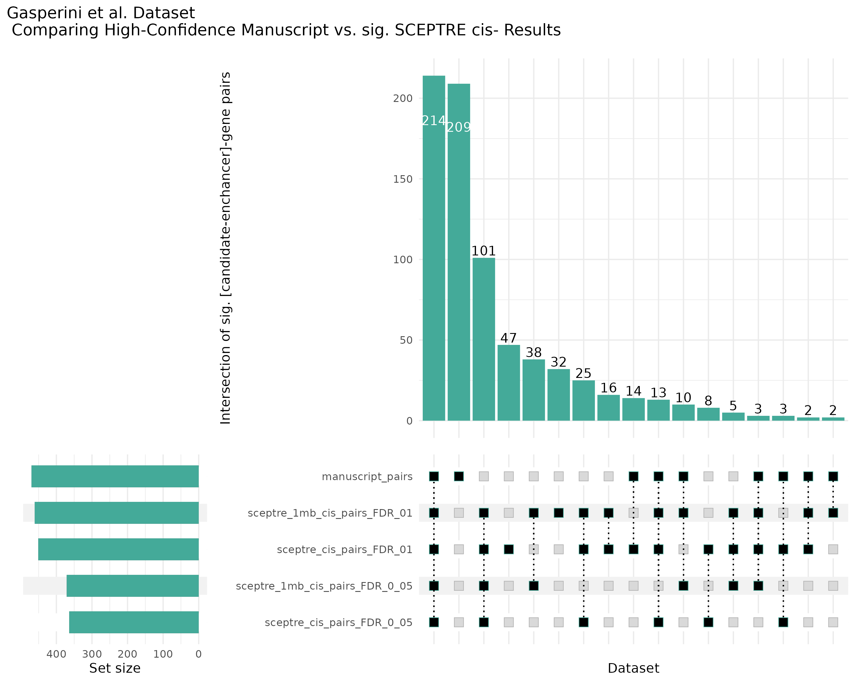
9/11/23 Comparison of Gasperini et al. cis- SCEPTRE and Manuscript Results
The goal of this section is to visualize the intersection of significant signals in the SCEPTRE cis- analysis of the Gasperini et al. dataset against the published manuscript results of 664 site-gene pairs of which 470 are high-confidence.
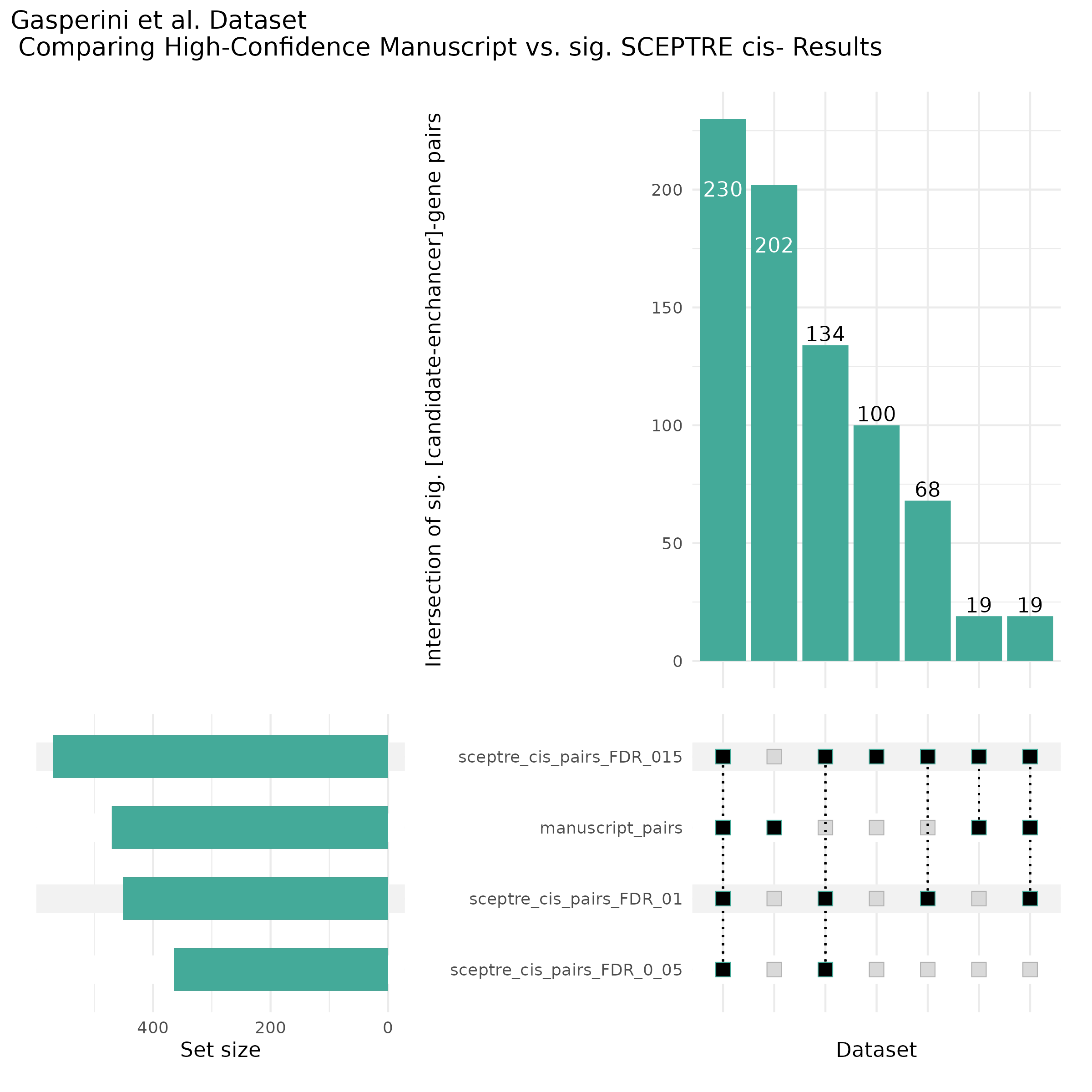
Additional cis- SCETPRE at cis- <= 1Mb and Different FDR corrections
8/30/23 Mappability Adjusted CellRanger with Intron Counts
This section repeats the analysis done below but on the Morris v1 dataset and uses a modified mappability correction method, it also includes average mappability of the high and low ratio selections.
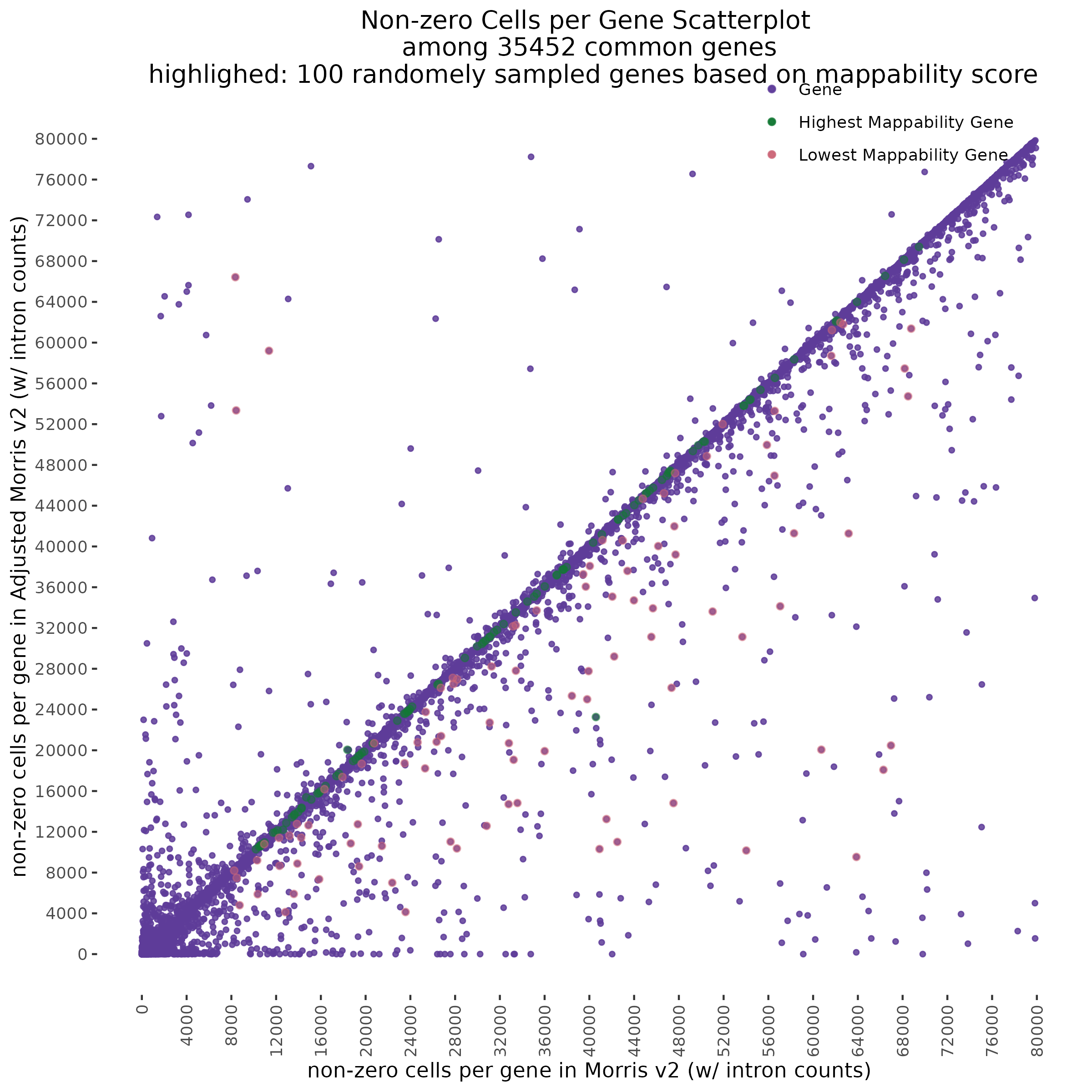
Highlights:
One question we asked was where will we find the highest and lowest mappability genes in the above scatter plot?
With QC filtering:
8/21/23 Mappability Adjusted CellRanger with Intron Counts
The purpose of this section is to analyze the effect of mappability correction with intron counting turned on in CellRanger software. For single nucleus data it is necesary to incude introns during quantification of expression counts from the raw underlying data. This means that including introns is a required setting for processing this data. This is due to the fact that reads from RNA captured in the nuclei will have a higher proportion of unspliced transcipts, as shown in K562 cells in a deep-sequencing study by Tilgner, H. et al. with some of the earlier work done by Ameur et al. (2011), who proposed co-transcriptional dominance in analysis of total RNA-Seq in cells from the human brain. While most splicing occurs during transcription in accoradance to the ‘co-transcriptional splicing’ model, some transcipts will be spliced later and will contain sequences mapping to intronic regions on the genome (introns). For example, Tilgner, H. et al. found alternative exons and long noncoding RNAs to have their splicing occur at a later time, with the latter sometimes not being spliced at all.
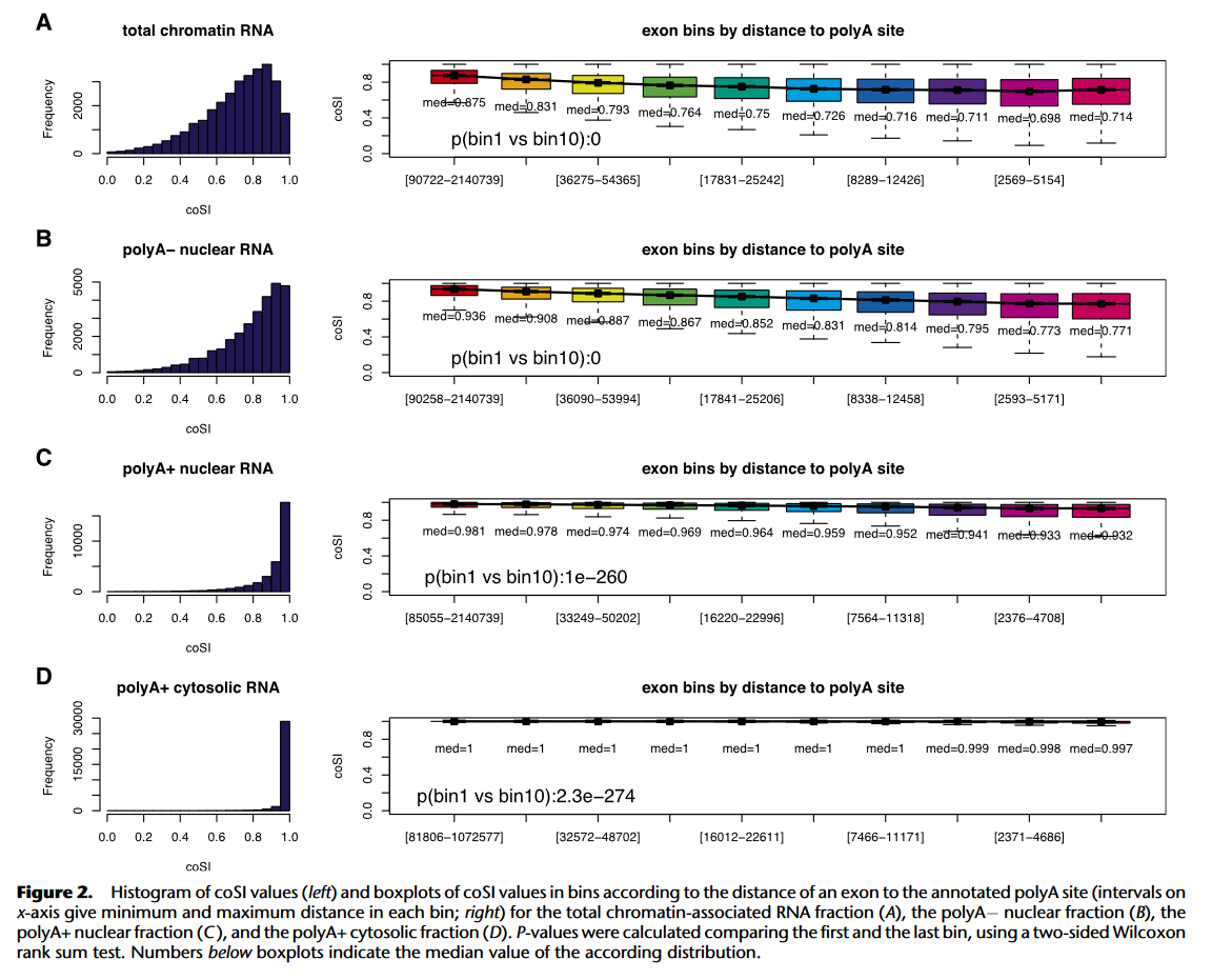
The Figure above shows that in K562 cells fractional analysis of deep RNA-Seq has shown that most splicing is initiated before completion of transcription due to the time the poly A site is reached in transcription and the markedly high coSI (author introduced score which represents the completed splicing index) of polyA- nuclear RNA shown in the above figure. This means that for single nucleus RNA-Seq we should expect a higher ratio of intron-aligning reads to exon-aligning reads.
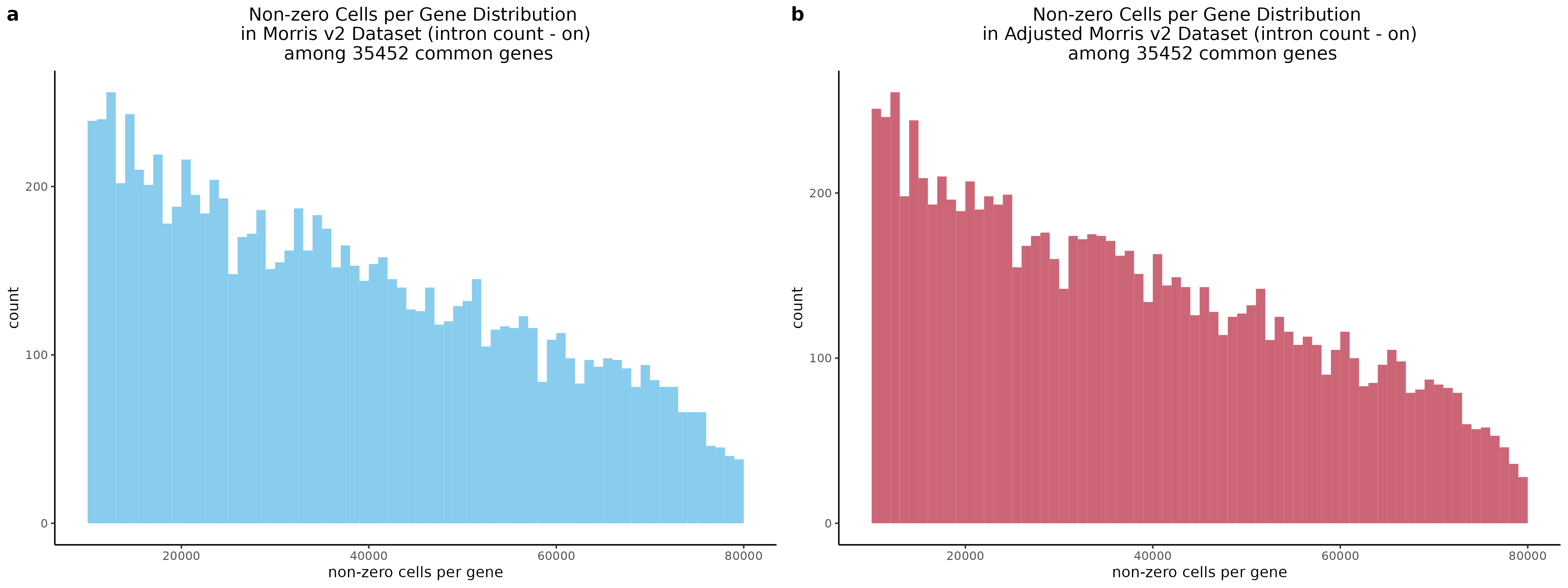
Evaluating Gene-Level Count Data in Morris v2 Dataset
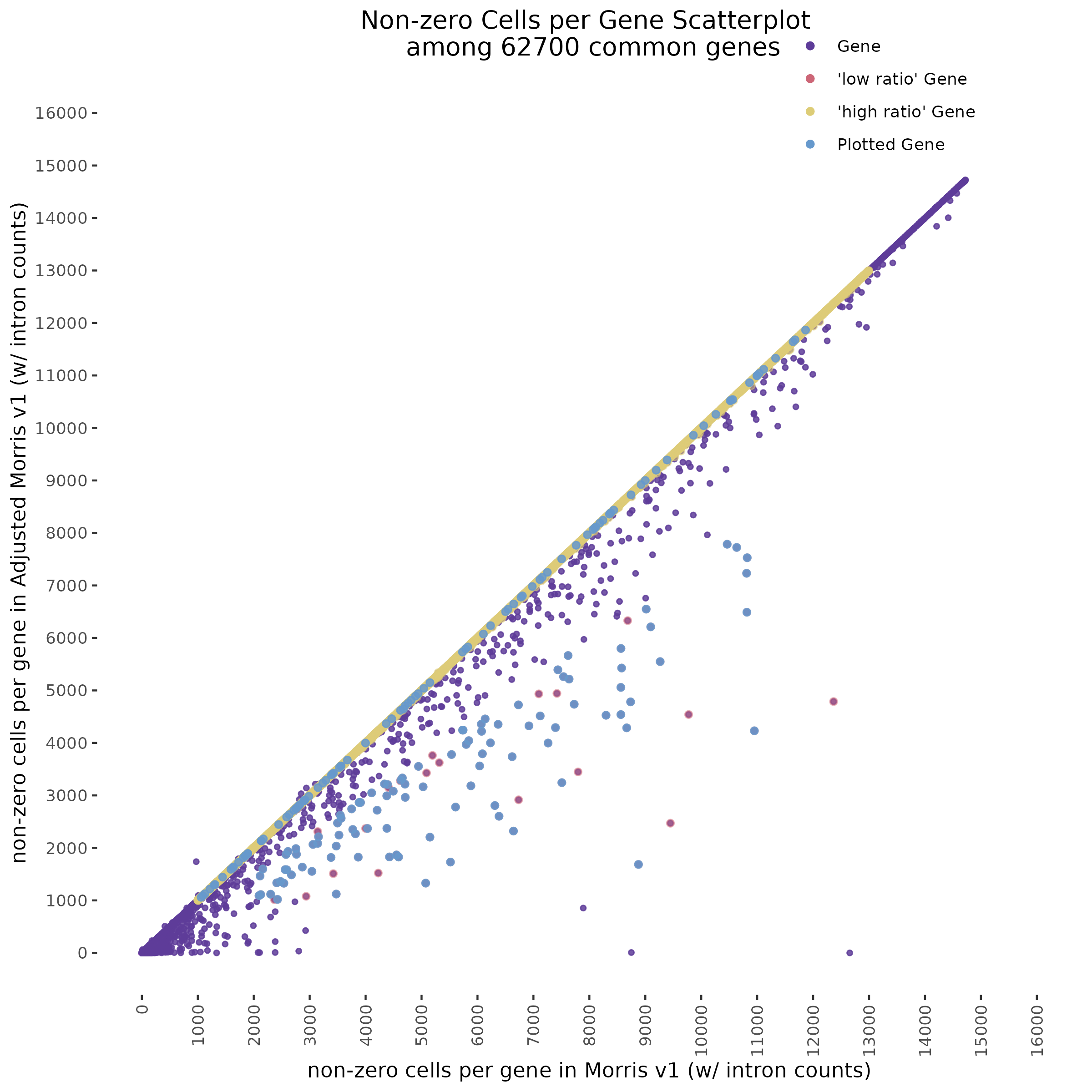
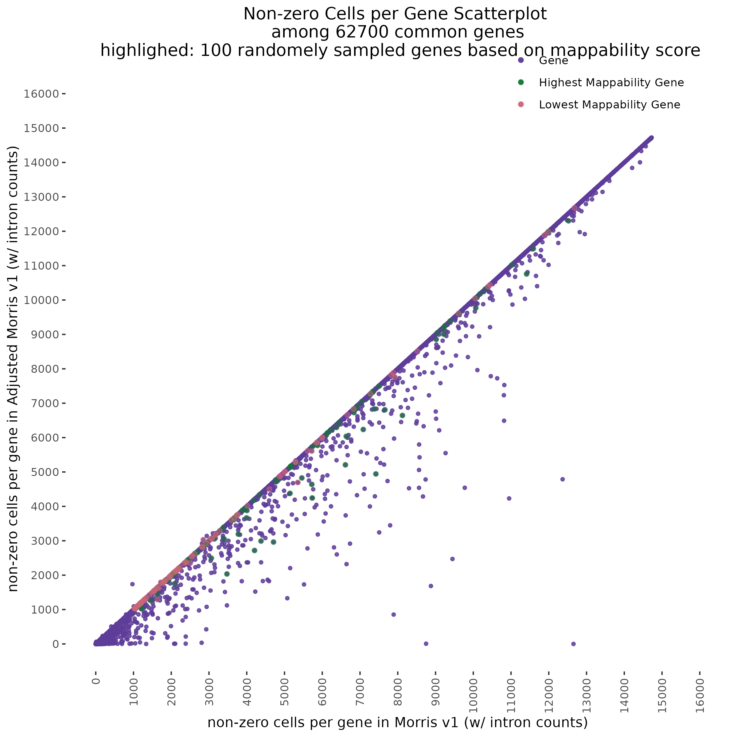
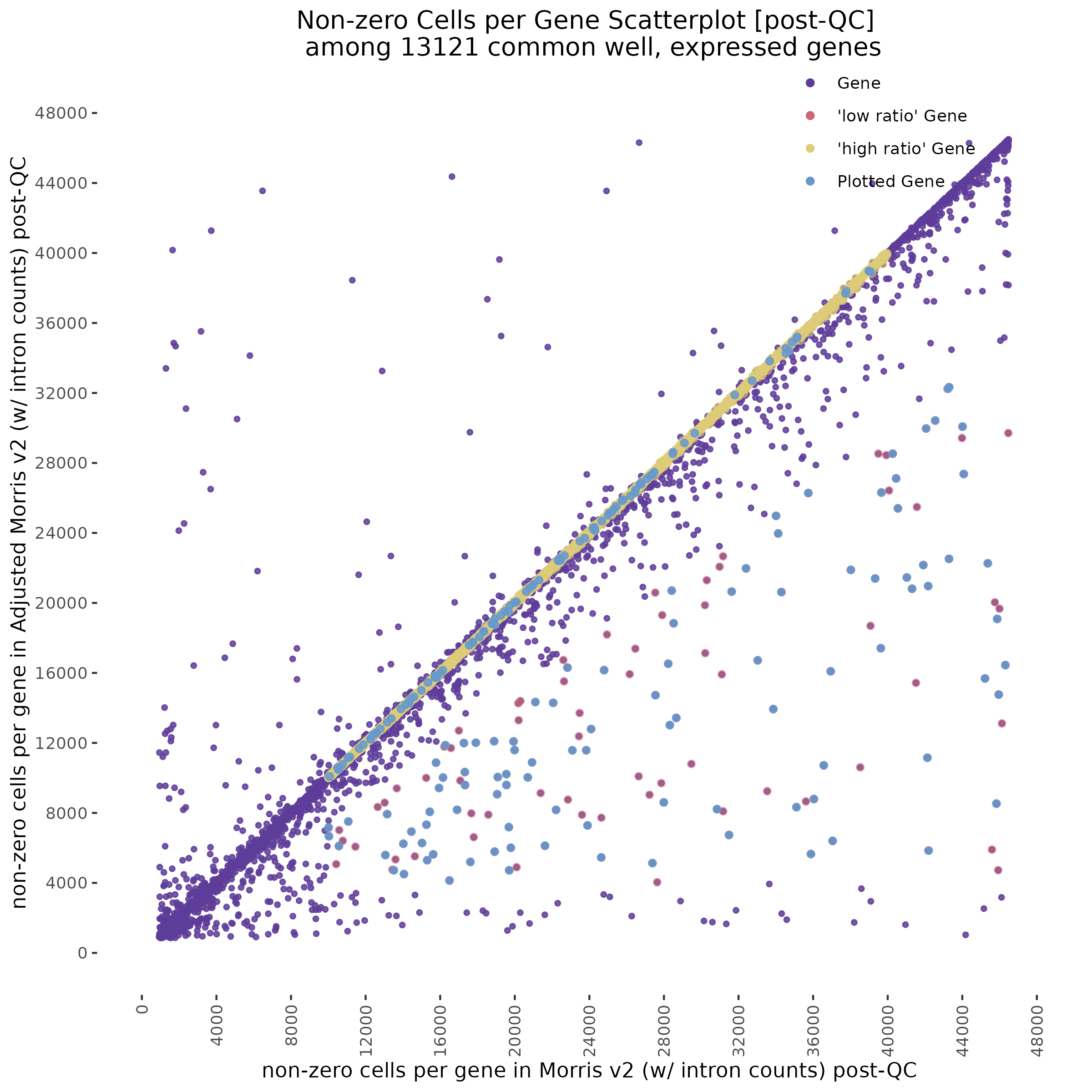
To start with a broad comparison, we plot and compare the shape of the distribution of non-zero cells per gene between the two datasets. The plot below shows that both the mappability adjusted and normal datasets have similarly shaped distributions.
In order to evaluate how the mappabiity adjustment performs we plotted the counts of non-zero cells per gene in both datasets, with each point corresponding to a single gene. We chose to compare non-zero counts becuase decreases in UMIs in a single gene accross a matched number of cells are easier to define by using a binary definition of change. We hypothesize that genes strongly affected by low mappability reads will likely contain a greater proportion of zero counts (UMIs).
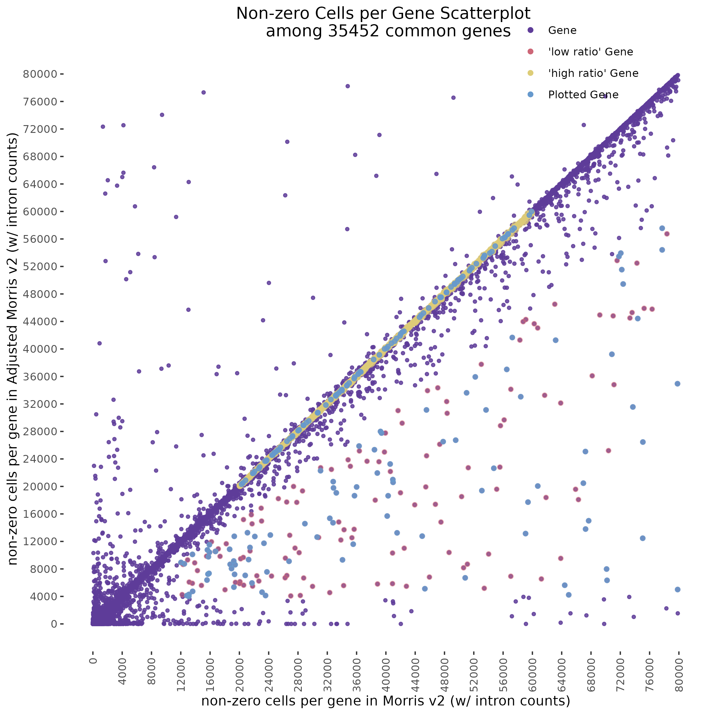
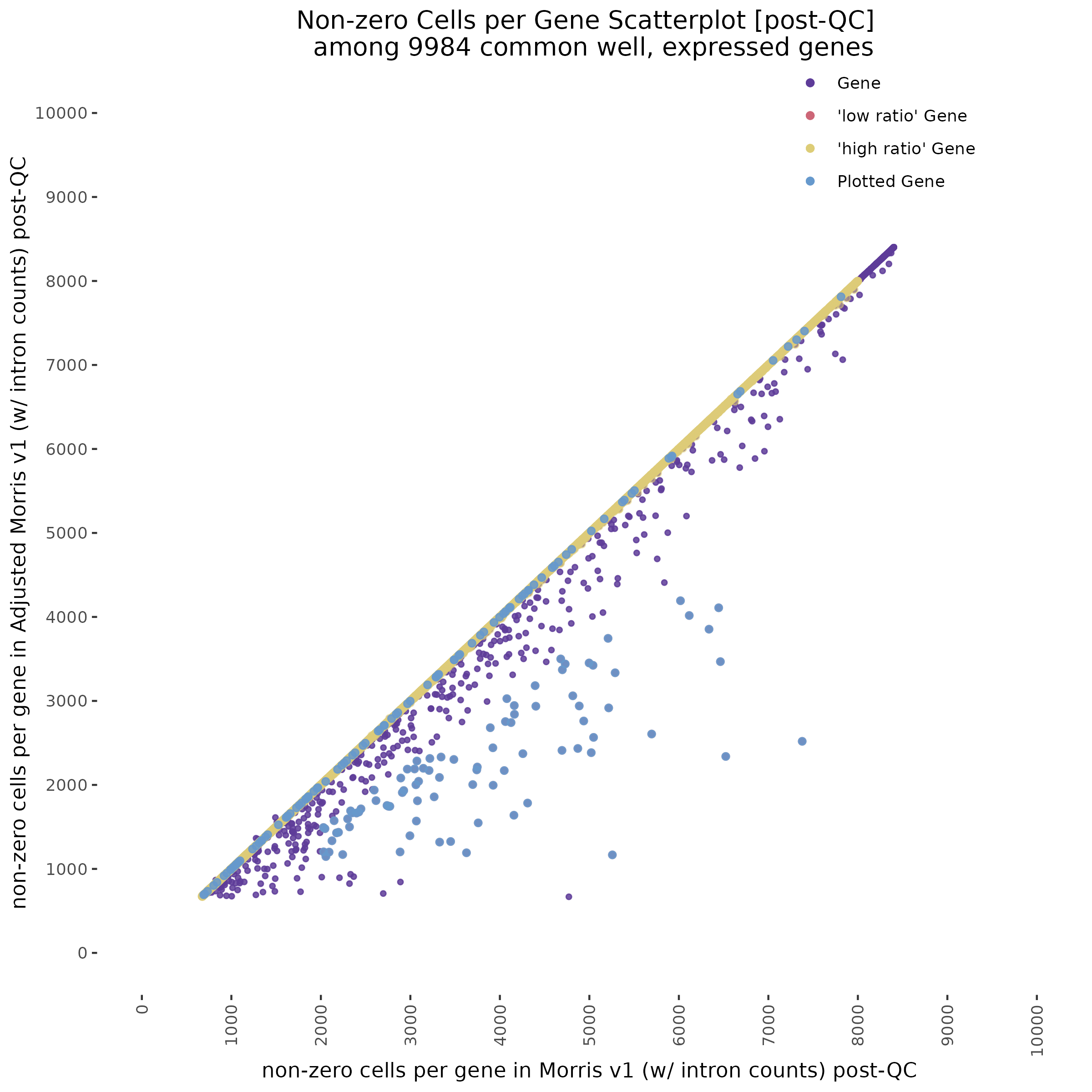
A Tale of Two Cities
In the plot above we highlight two different sub groups in the plot. The ‘high ratio’ genes in gold represent genes where the ratio of non-zero cells per gene was between 0.01 of 1.0 (0.99<ratio<1.01) or nearly identical between datasets. While the ‘low ratio’ genes highlighed in red represent genes where the ratio of non-zero cells per gene decreased between mappability adjustedment and was less than 0.75, the genes also must have had non-zero counts above certain dataset specific thresholds. This was done in order to capture a good ‘triangular shaped’ sample of genes that are well expressed in both datasets but contain deffering non-zero cells between datasets due to mappability adjustment.
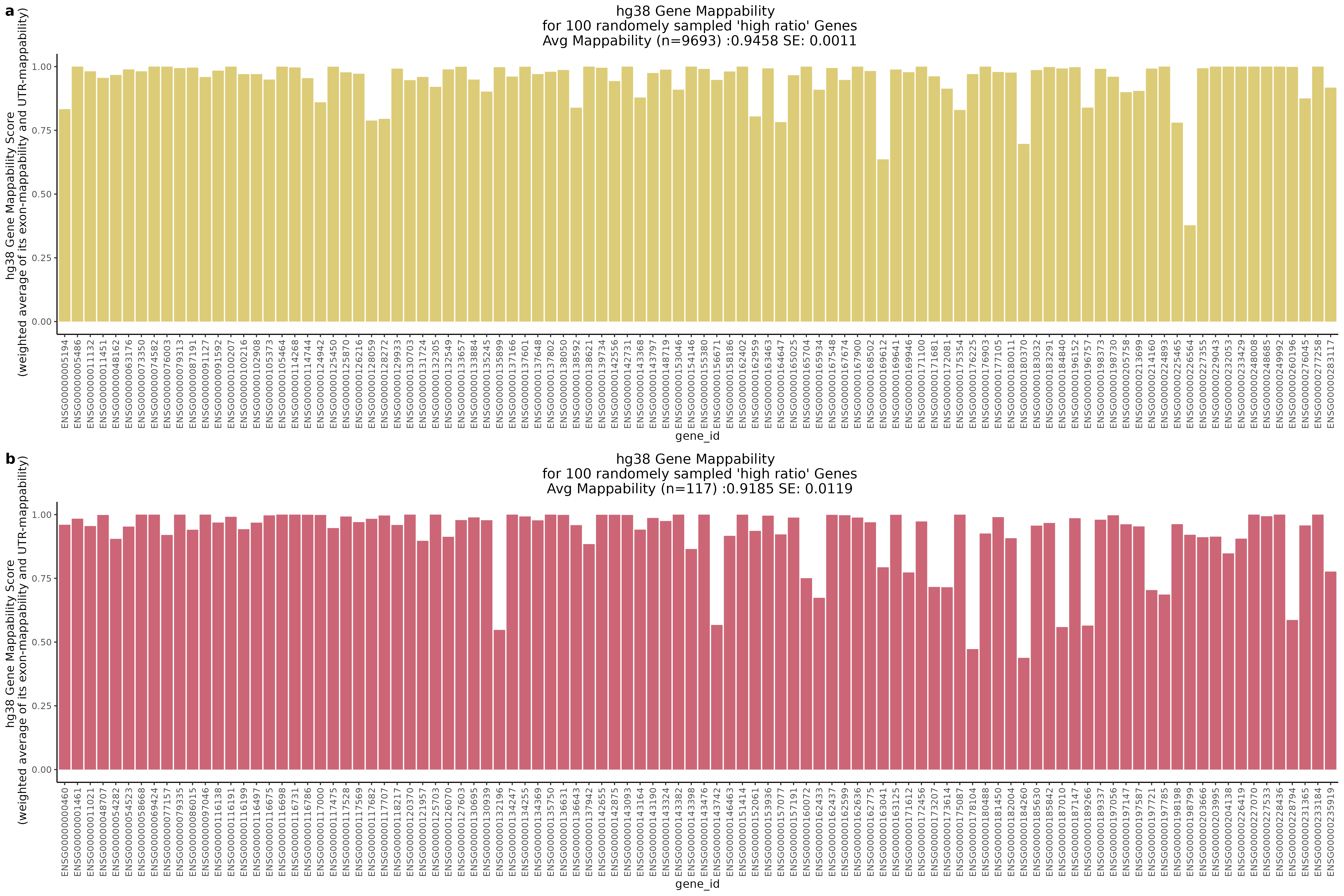
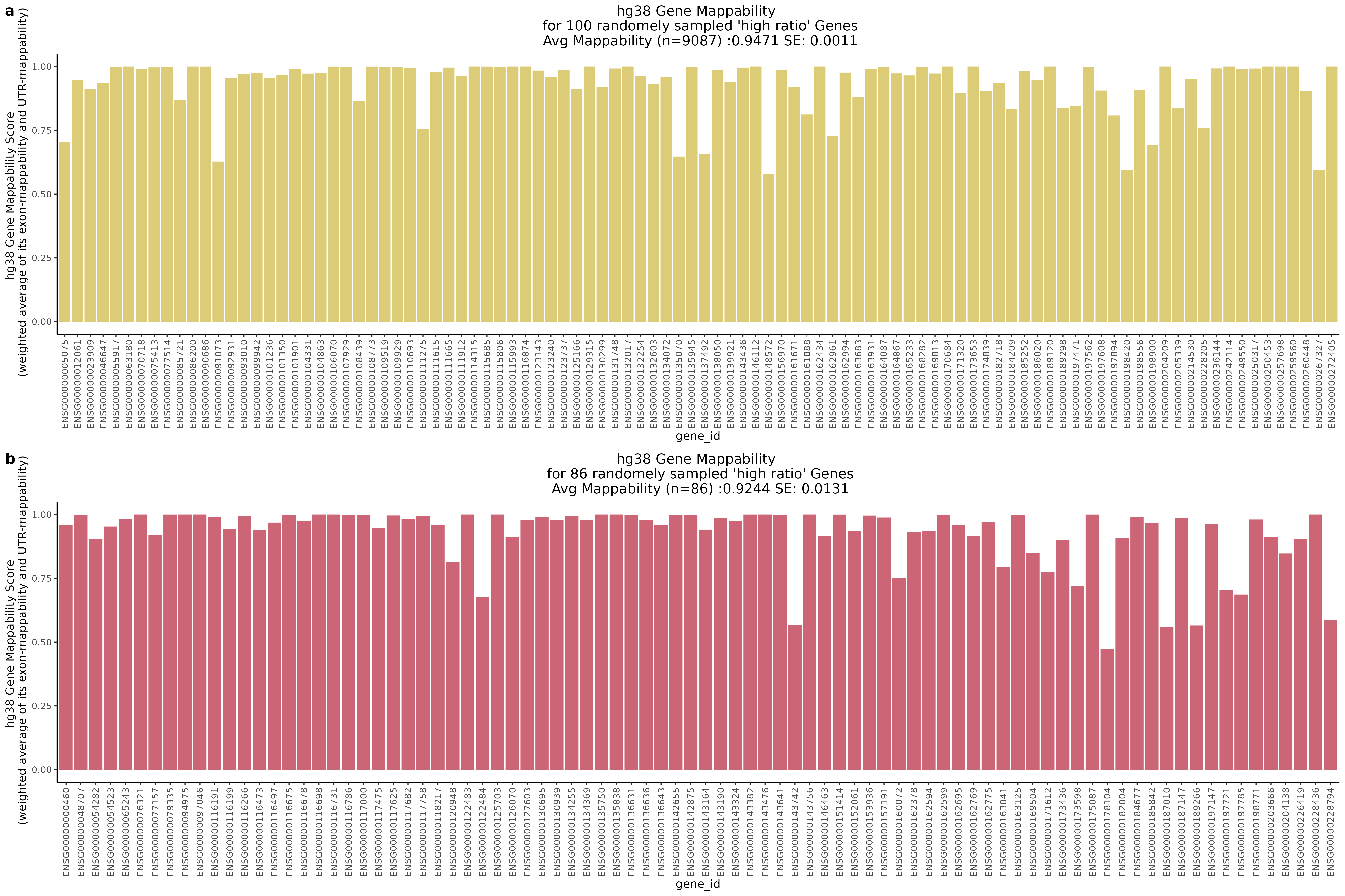
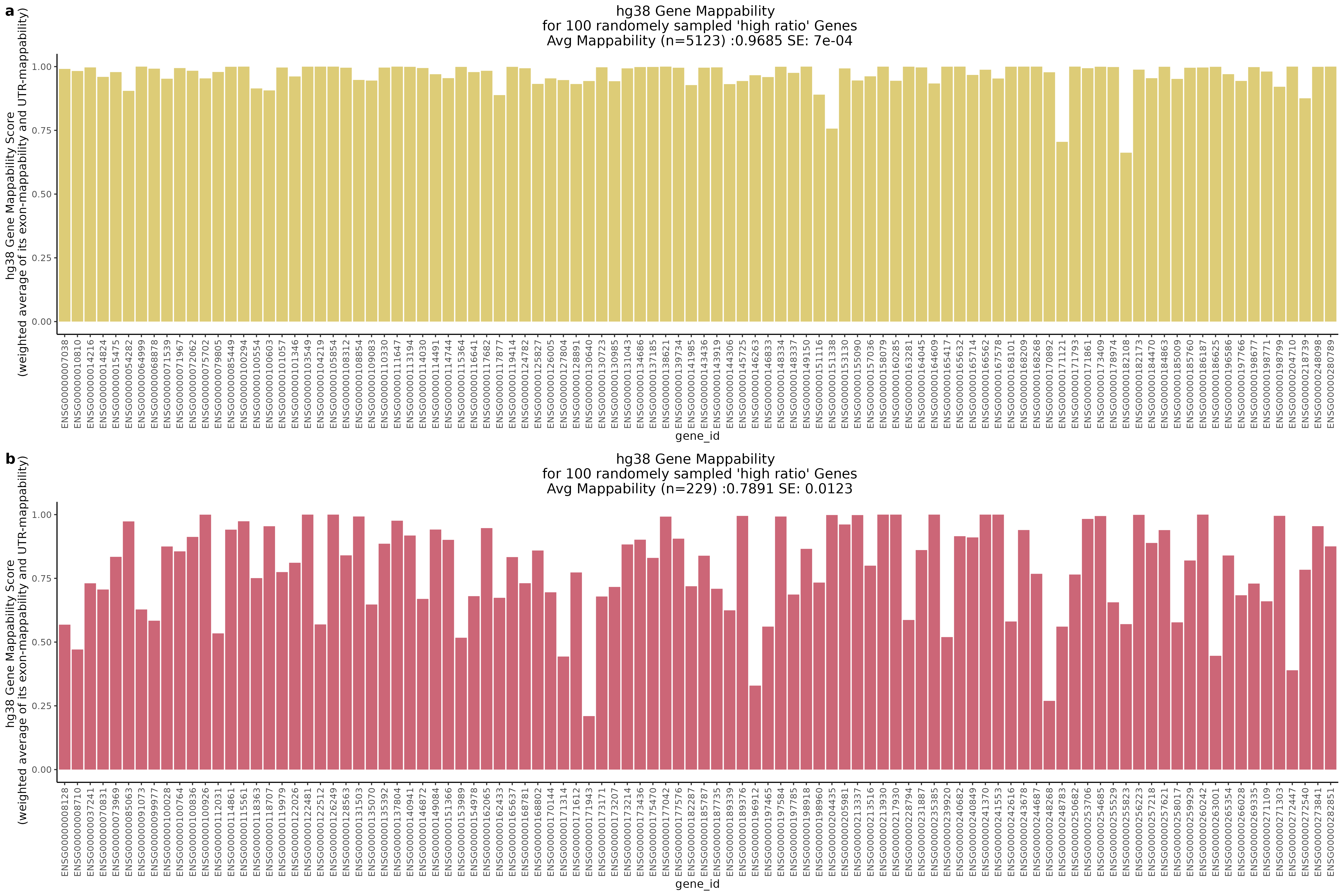
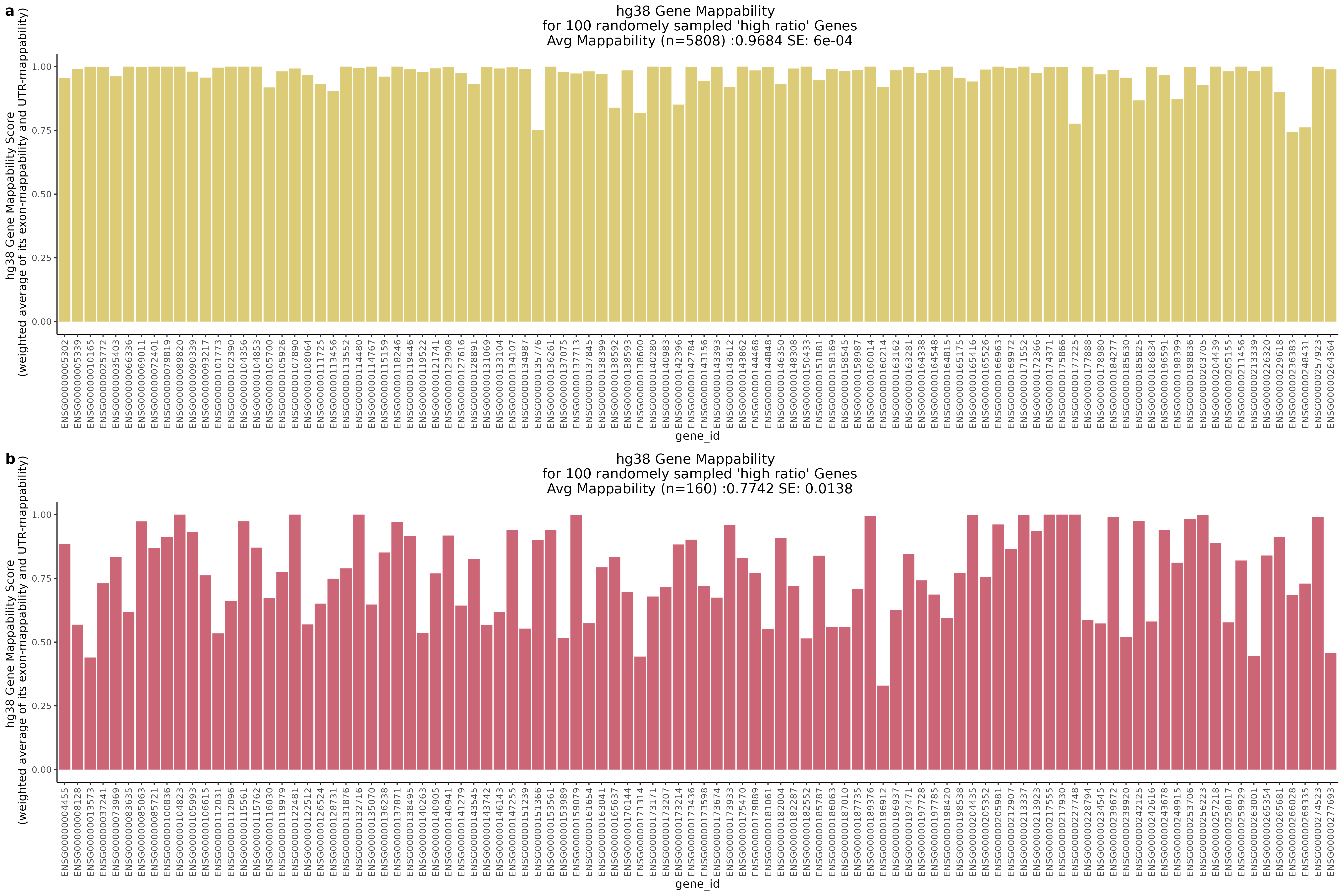
One question that we wanted to answer was wether the low ratio or high ratio genes highlighted in the plot above had differing gene mappabiity scores. It would follow that differences in non-zero cells per gene in genes affected by low mappability reads would affect genes with lower mappability scores. We therefore expect to see a decrease in gene mappability when comparing ‘high ratio’ genes to ‘low ratio’ genes. In order to demonstrate this we randomely sampled 100 of each of the highlighted subgroups and plotted their gene mappability scores as defined by Alexis Battle and Ashis Saha 2018. The gene mappability scores used were defined as “weighted average of its exon- and UTR-mappability, weights being proportional to the total length of exonic regions and UTRs, respectively” (Alexis Battle and Ashis Saha 2018). A gene-mappabiliy score of 1 represents a gene where are the k-mers are uniquely mapped to that gene, and no other regions on the genome.
Highlights:
One question we asked was where will we find the highest and lowest mappability genes in the above scatter plot?
With QC filtering:
Repeating this analysis using QCed matrices for both datasets shows similar results. Below, the datasets were subject to cell filtering and gene filtering to identify and compare common well-expressed genes against matching cells in post-qc data.
8/21/23 Gaserperini Split Analysis
This section presents the results of running SCETPRE trans- analysis on random subsets of the Gasperini data. Specifically we are interested in comparing the results from the 50% random cell subset and the 70% random subset. Here we perform normal cell QC but we then randomely sample 50 or 70 percent of cells prior to perfoming gene and guide QC. This results in a downsampled dataset where genes and guides are affected by the decrease in total cells availible for analysis.
UpsetR Plot of Signals between 3 Gasperini cis- SCEPTRE datasets
This is the cis- pair analysis. 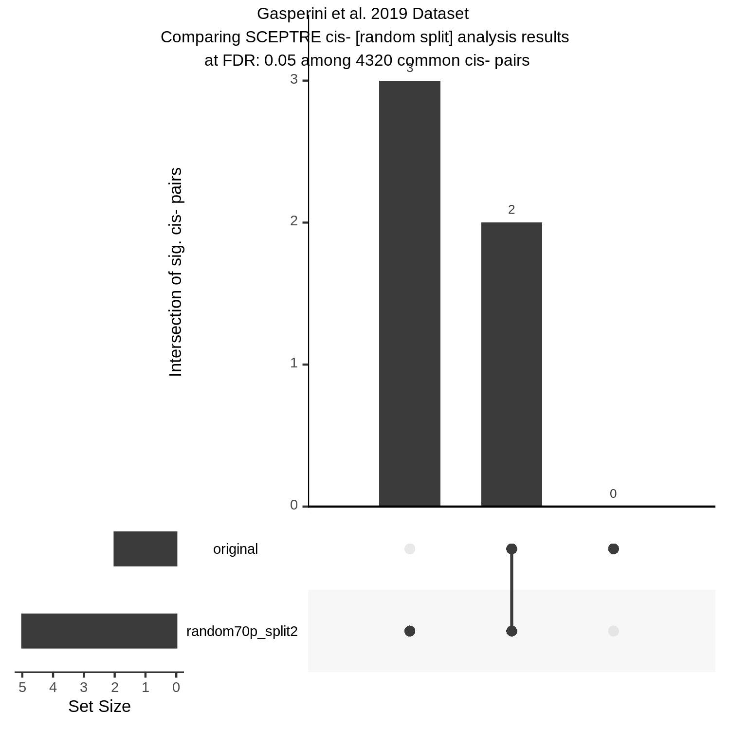
UpsetR Plot of Signals between 3 Gasperini trans- SCEPTRE datasets
This is the trans- pair analysis. ![]()
There may be an issue with these results, I am in the process of running a few checks.
8/21/23 SCEPTRE Replication & pi1 Replication in DNG eQTL
The purpose of this section is to report on SCETPRE replication and replication pi1 stat in order to look at scRNA Seq and SCEPTRE’s ability to replicate eQTL signals found in the DGN study, bulk tissue eQTL vs scRNAseq w/ CRISPR perturbationsa at the eGene site.
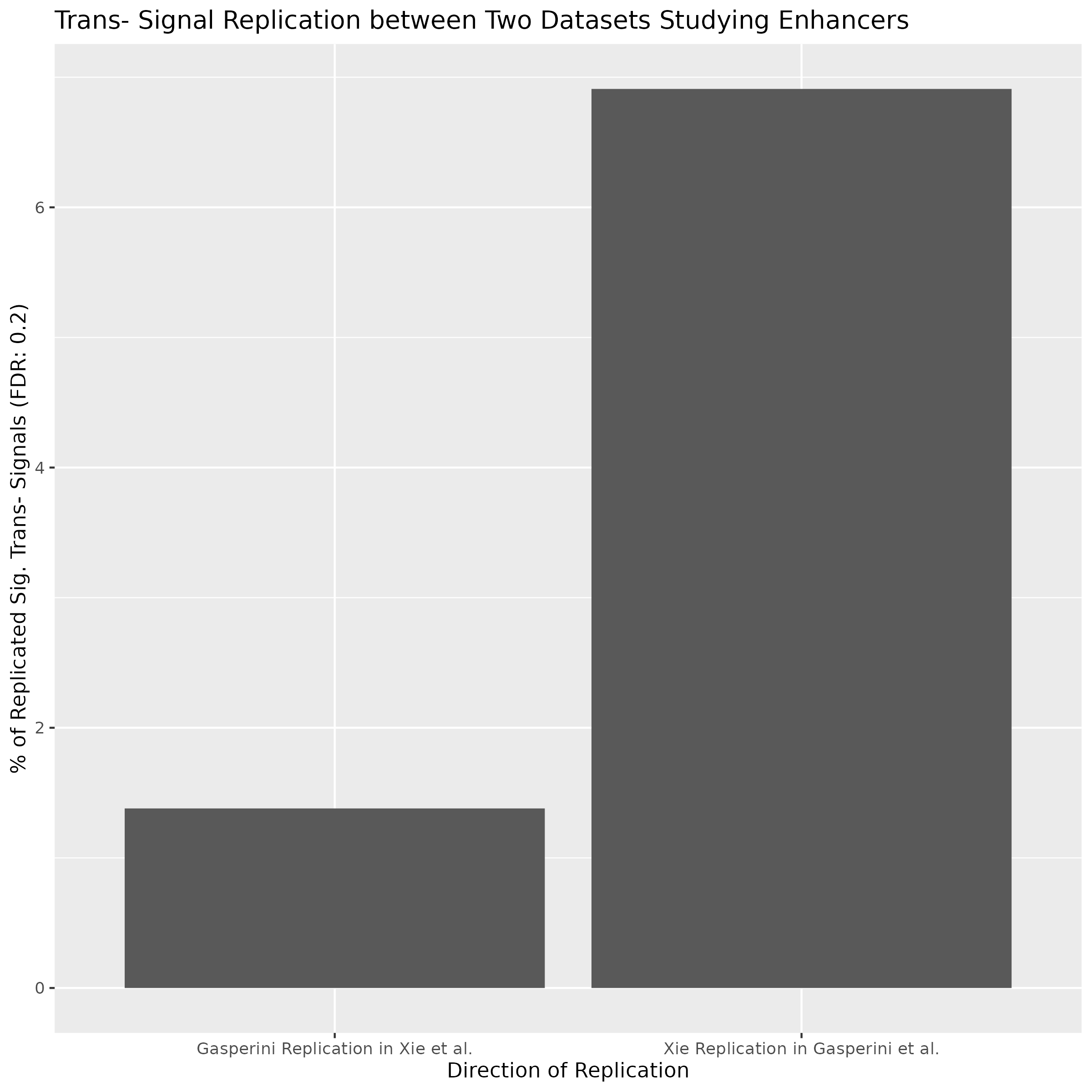
Replication within SCEPTRE
To evaluate SCETPRE between set in scRNA datasets we compared trans- signal replication between Xie et al. and Gasperini et al. The % of replicated significant trans- signals is shown on the y-axis while the direction of the replication comparision is indicated on the x-axis of the barplot.
pi1 Statistic for Replication between eQTLs in DGN and SCEPTRE
- The pi1 between DGN and Xie et al dataset. is 0.06414
- The pi1 between DGn and Gaserperini et al. dataset is 0.4092
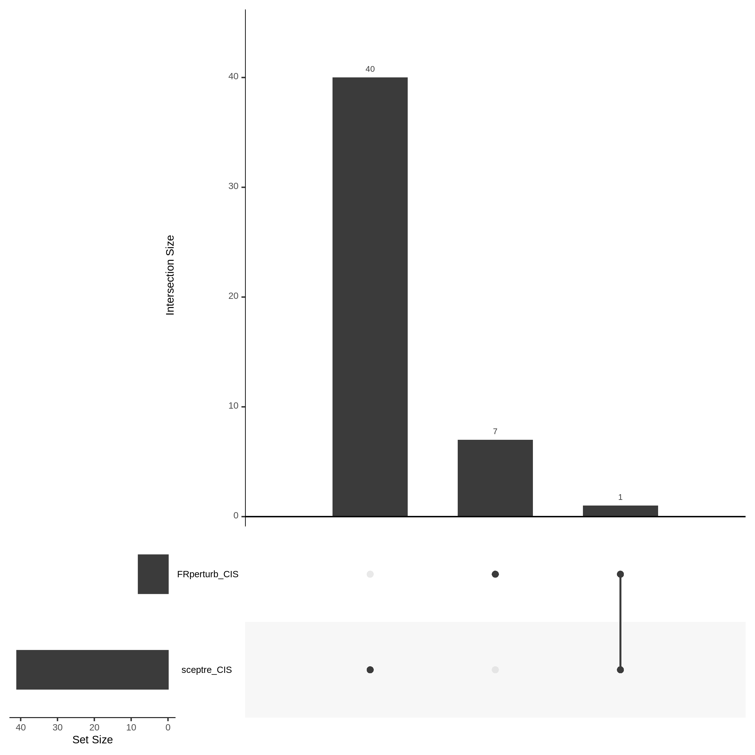
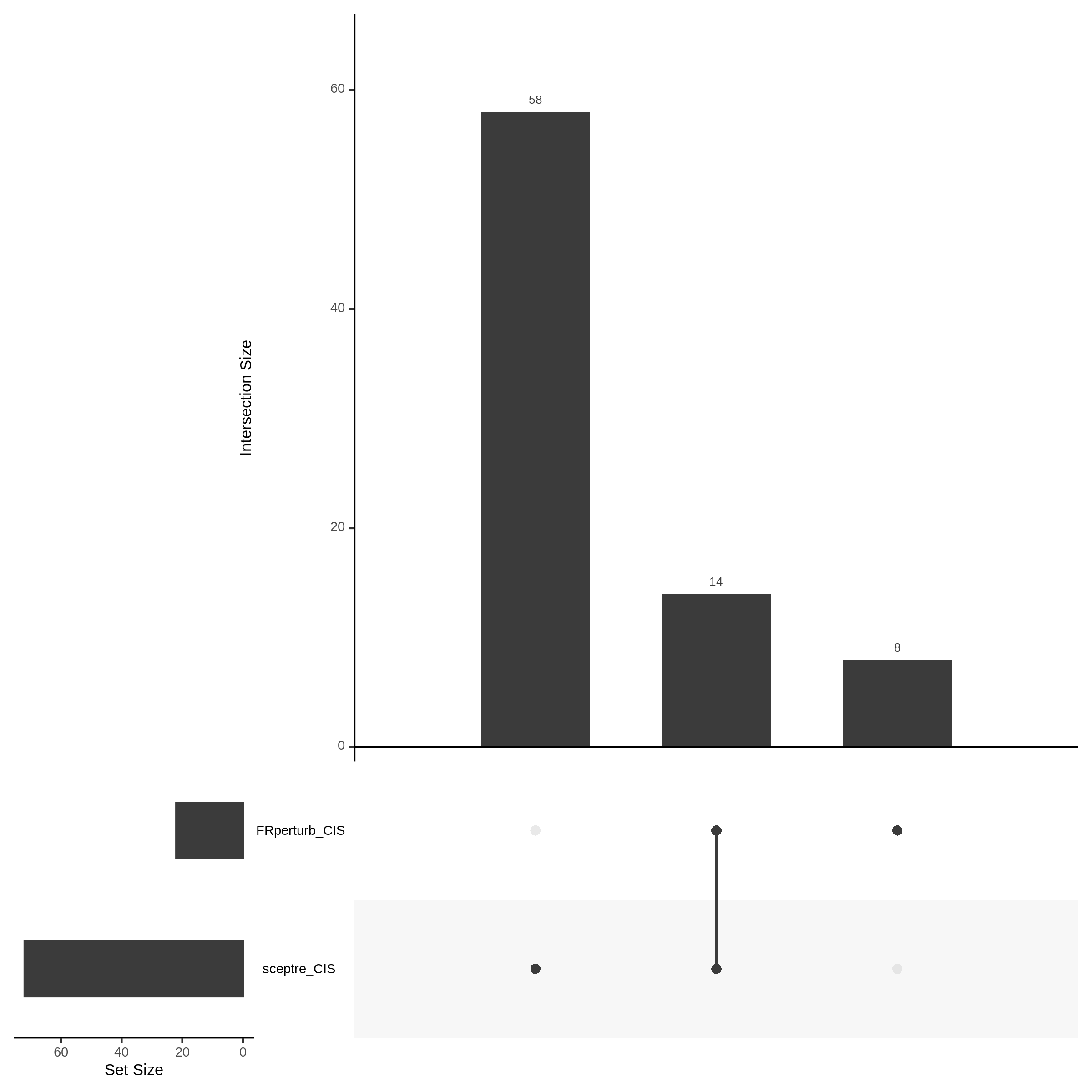
7/12/23 UPSETR Plots Comparing Preliminary FRPerturb v SCEPTRE
This section will showcase the results of comparing FRPerturb to SCETPRE in datasets with respect to the cis analysis. The UPSETR plots below show the intersection between significant (FDR < 0.1) FRPerturb results and SCETPRE.
For the Morris v2 dataset there are 4,438 cis pairs and SCETPRE found 42 signals, 41 regulators at an cis FDR of 0.05. At the same FDR, FRPerturb found 16 signals, 8 regulators. Below is an UPsetR plot between the 41 sig. cis regulators in SCETPRE and 8 regulators in FRPerturb.
For the Xie et al. dataset there are 2,727 cis pairs and SCETPRE found 95 signals, 72 regulators were significant at an cis FDR of 0.05. At the same time, FRperturb found 54 signals and 22 regulators.
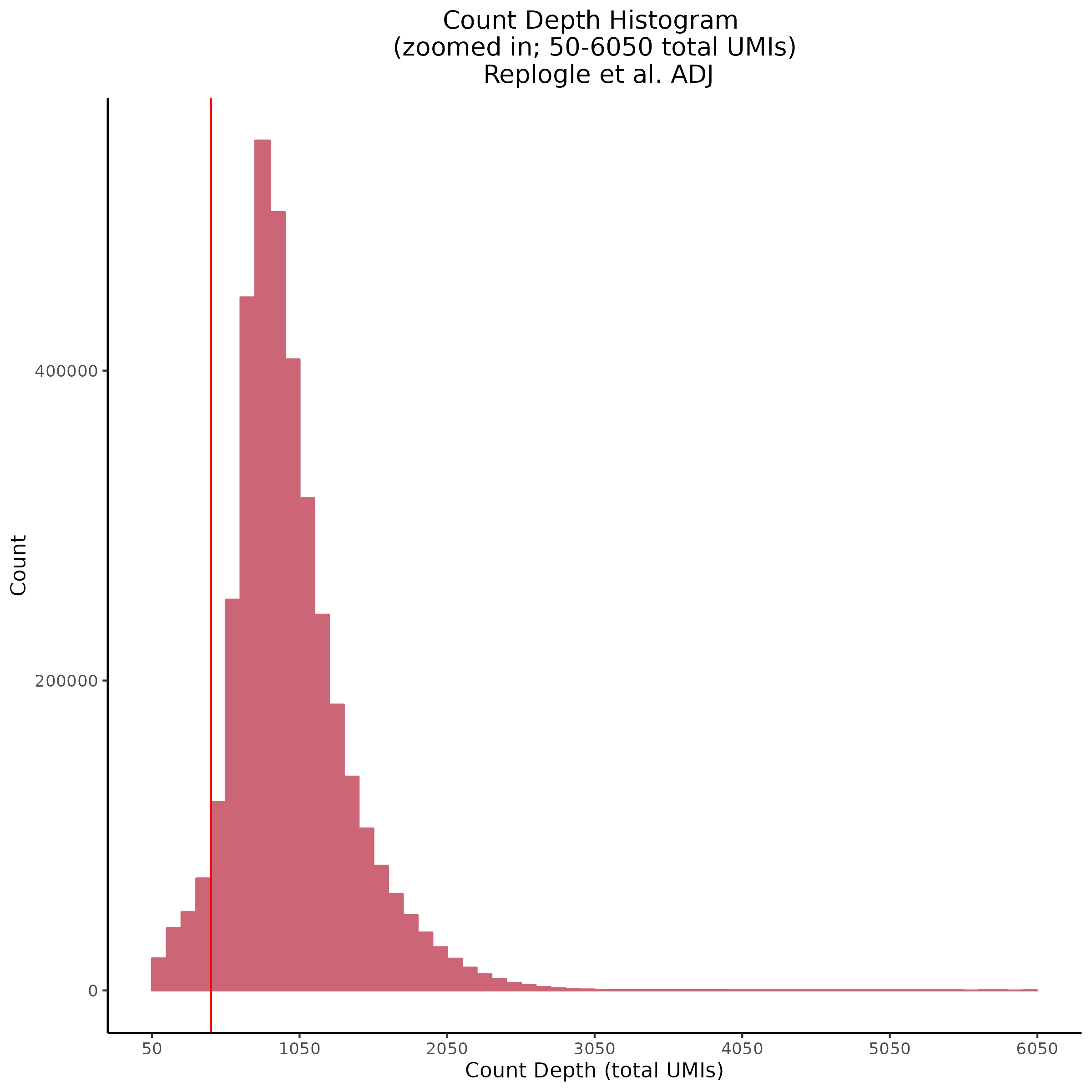
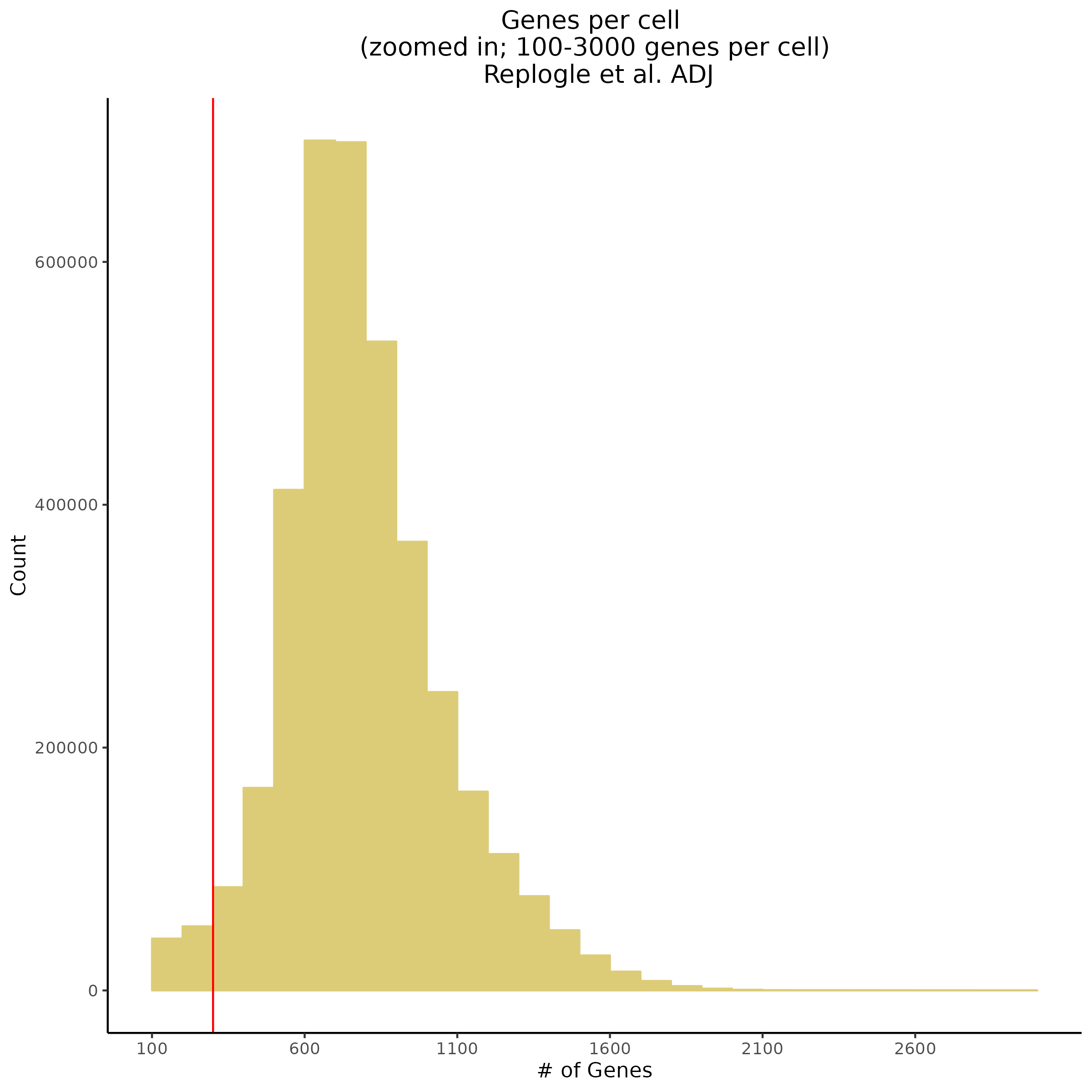
7/12/23 Additional Replogle QC
One thing that has come to attention is the fact that after normalization the amount of genes per cell and overall count depth (total reads) per cell is severely low. This makes increasing the QC parameters of the entire dataset after count depth normnalization not possible.
For example here is the overall shape of the distribution of both genes per cell and count depth after normalization in th ecurrent dataset. The red vertical lines inicate current QC parameters.
In order to investigate the cause of the post-normalization criteria we can try plotting pre-normalization stats per gemgroup (aka per batch):
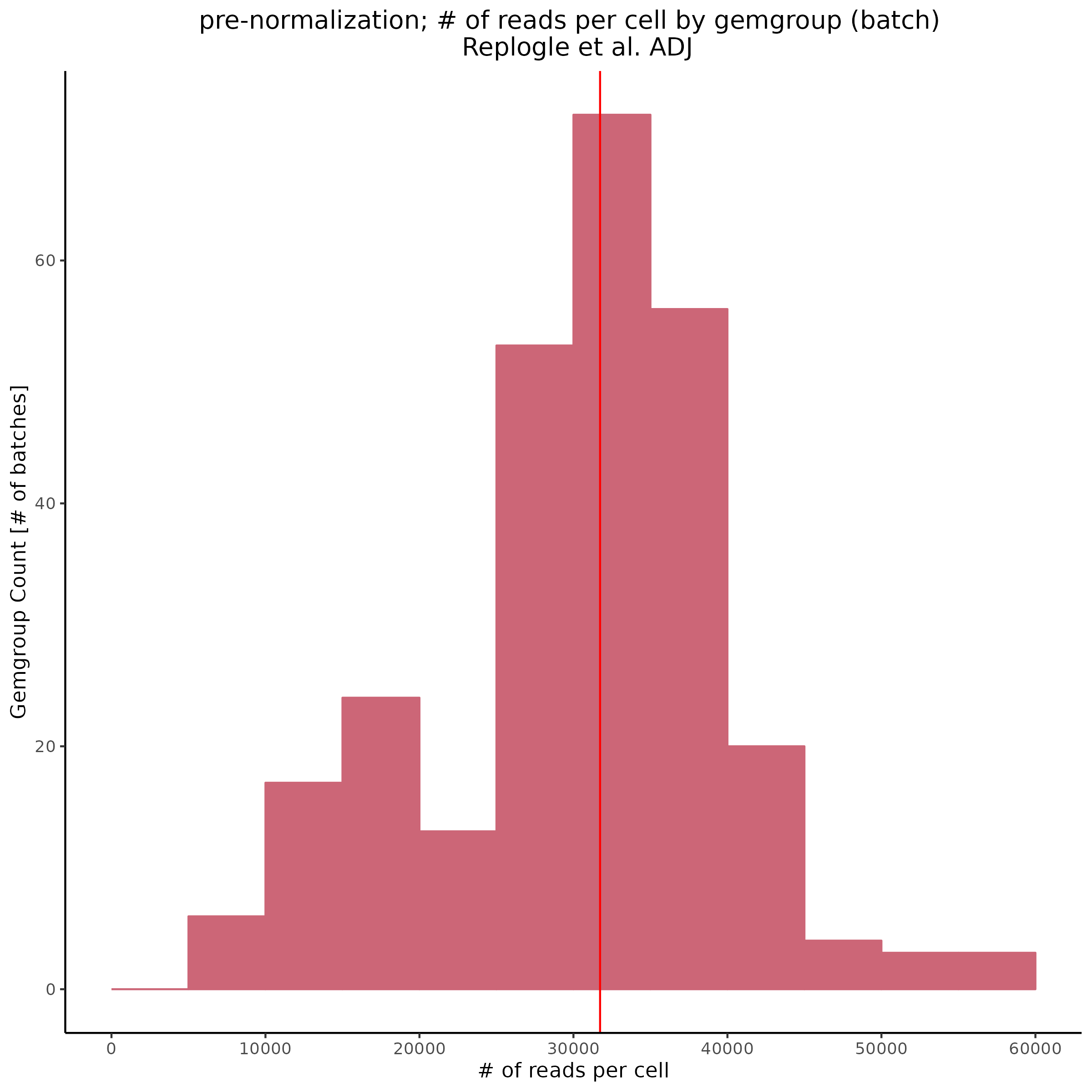
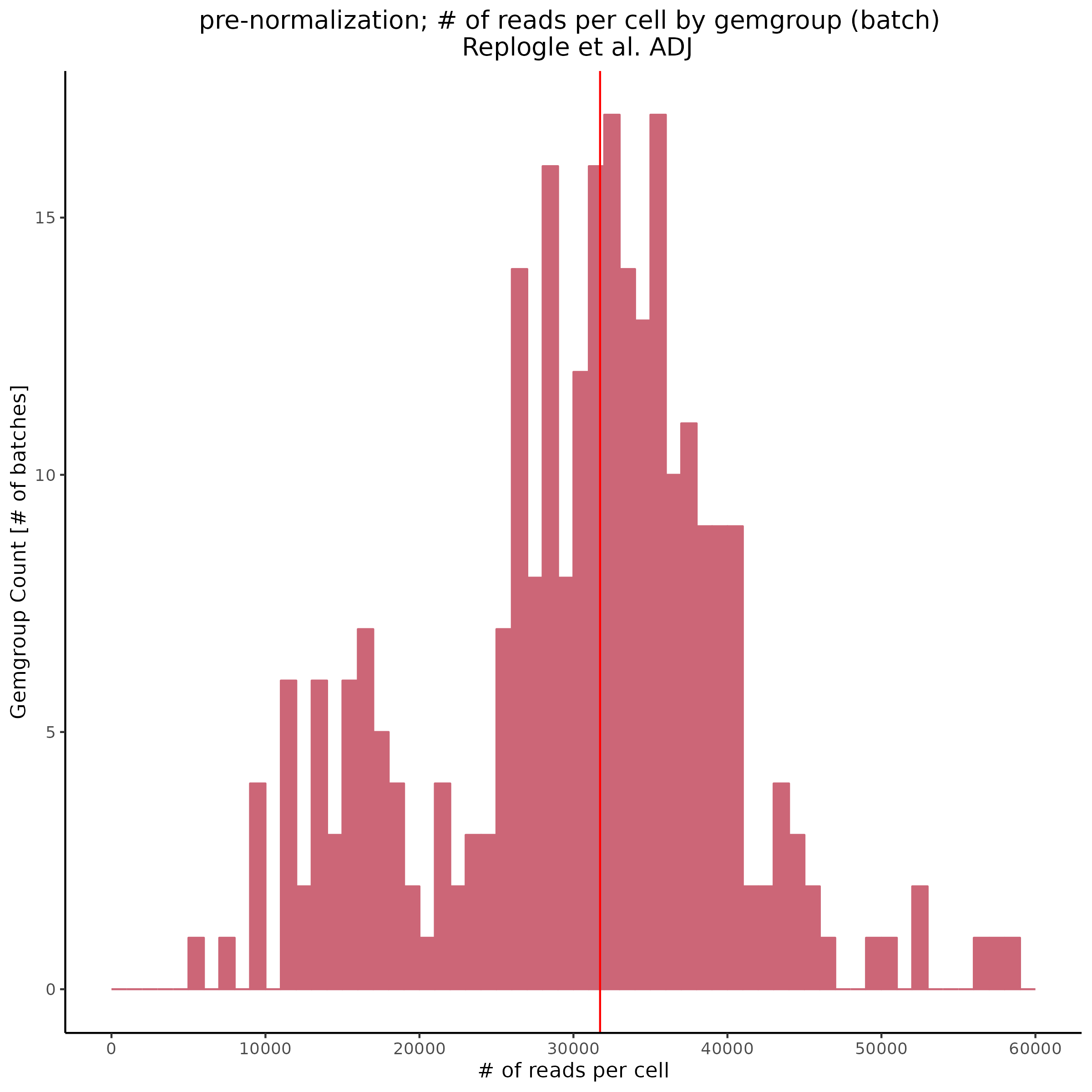
Also showing the same patterns in the feature reads per cell (per gemgroup/batch):
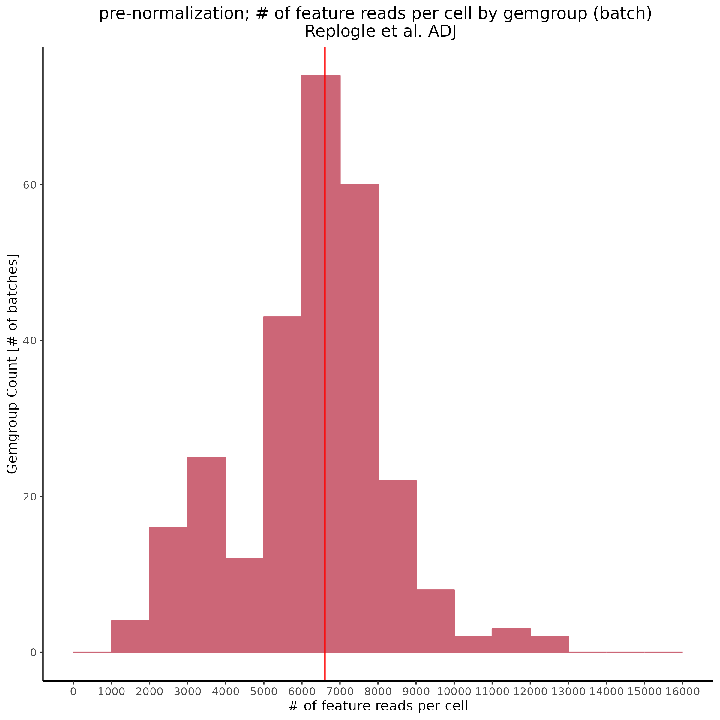
Overall it seems that some batches in the KD8 dataset differ significantly from other batches before normalization. This could be the cause of the low gene per cell count/ low overall count depth after normalization.
6/12/23 GO Term Analysis of 4 trans- SCEPTRE in 3 Datasets
In this section we will examine the FDR significant regulators within the trans SCEPTRE results of 4 runs (Morris v1, Morris v2, Xie, and Gasperini).
Annotation of Regulators in Results
In order to test for significant enrichment of GO terms associated with biological processes, we need to first annotated our significant results since our trans- regulators in these 3 datasets refer to sgRNAs targeting both enhancers and SNPs. To address this we will link each sgRNA in the trans- gRNA-gene pairs to the closest protein coding or lncRNA gene based on the gencode v32 reference.
# the references used
protein_coding_gencode32 = readRDS('./gencode.v32.primary_assembly.annotation.protein_coding.rds')
protein_coding_lncRNA_gencode32 = readRDS('./gencode.v32.primary_assembly.annotation.protein_coding_lncRNA.rds')
Both of these references are sourced from the GENCODE V32 GTF reference file. The R code to replicate and create these references is availible REFERENCE CODE
GO Term Results for Protein Coding /w lncRNAs added (n=36,843 genes)
For all sig. trans- regulators the results can be seen here: All trans- regulators (n=993)
GO Term Results for Protein Coding (n=19,994 genes)
For all sig. trans- regulators the results can be seen here: All trans- regulators (n=922)
5/17/23 Gasperini et al. and Xie et al. Mappabiity Adjusted QC
This section will breifly show the basic QC parameters set to filter the mappabiity adjusted version of two of our primary datasets.
- This update features a more careful approach to plotting since we need to make sure that each QC variable is specific to the dataset
- This QC also features a major correction: previously there was a mistake which resulted in filtering to avoid zeros in one of the covariates. The thresholded, unique gRNA/guide covaraite has now been removed, which only the total gRNA UMIs as a covariate.
Gasperini et al. Mappability Adj. QC:
Xie et al. Mappability Adj. QC:
4/26/23 Gasperini QC
This section goes over the QC that was performed in order to prepare the Gasperini dataset for SCEPTER analysis using our QC pipelione.
One of the key modifications to the pipeline inludes the usage of the Suerat in order to read the 10X H5 output of CellRanger Aggr. It is also important to note that in order to aggregate the Gasperini dataset both the lab node and the multicore CellRanger software needed to be used.
Gasperini Dataset Breaks the Normal workflow
This section rehashes what was briefly discussed above: which is that the Gasperini dataset is already large enough to warrant two major changes:
- Better to use H5. H5 is a much denser and more effective way of storing count matric data. CellRanger outputs this result as the filtered H5 in the outs folder. For larger datasets it seems imperative to use the H5 files while working with the raw data.
By changing the Gasperini QC to use H5 matrices we can achieve reading GEX/GDO matrices + grouping the guide matrix in 8 minutes.
[1] "combined matrix size: "
[1]   2447 246076
473.602 sec elapsed- Use of the modified 10X CellRanger software. It became necessary to aggregate the dataset with a multicore protospacer counting code becuase the dataset even of this age (2019) contains too many guides.
For example, when running with the modified 10X Cellranager we can achieve aggregation in 25hr of compute time. And importantly, I found that the processing time was spend almost entirely on the multicore protospacer count step:
2023-04-11 13:25:42 [runtime] (update)          ID.AGG_Gasperini.SC_RNA_AGGREGATOR_CS.COUNT_AGGR.SC_RNA_AGGREGATOR._CRISPR_ANALYZER.CALL_PROTOSPACERS.fork0 chunks_running
2023-04-12 13:09:30 [runtime] (chunks_complete) ID.AGG_Gasperini.SC_RNA_AGGREGATOR_CS.COUNT_AGGR.SC_RNA_AGGREGATOR._CRISPR_ANALYZER.CALL_PROTOSPACERS
From these logs we can see that the protospacer time is ALMOST 24 hours! The total runtime is just larger than 25 hours so we can eviudently see that protospacer counting and aggregation takes a super long time even for a smaller dataset with a lot less cells than Replogle (3.9m cells, 8 days aggregate time)
Gaserperini QC Plot Results
One thing to note is that these plots are now standard for our pipeline with every dataset subject to these views/plots to set QC thresholds (dataset specific). These plots show the data prior to filtering but place RED lines where the current QC thresholds will be applied as a result of QC.
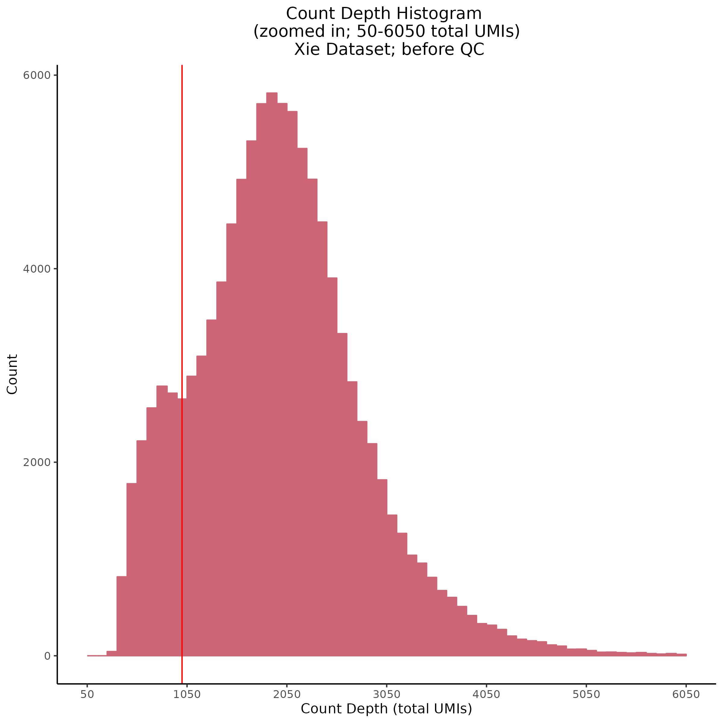
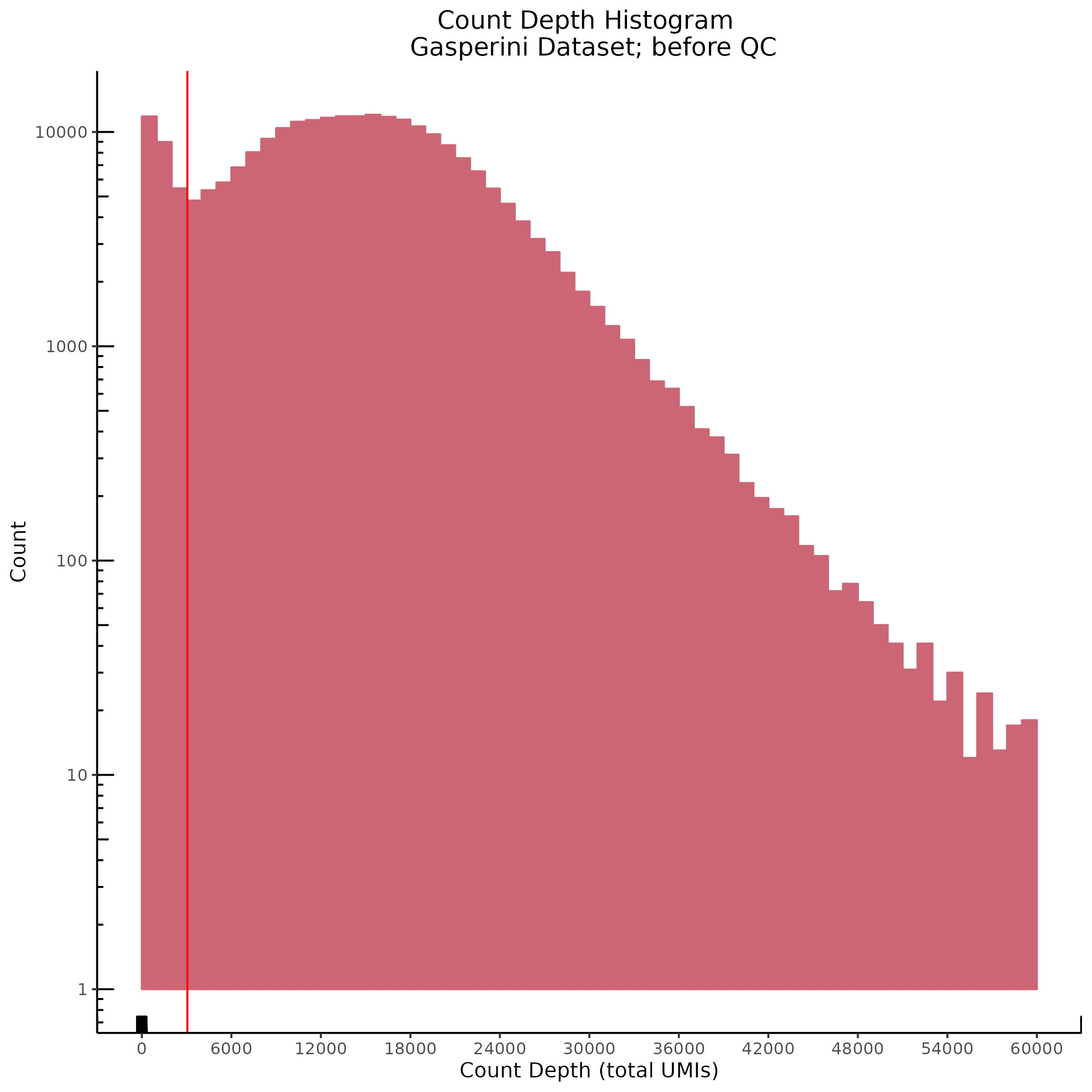
Count Depth (total UMIs per cell)
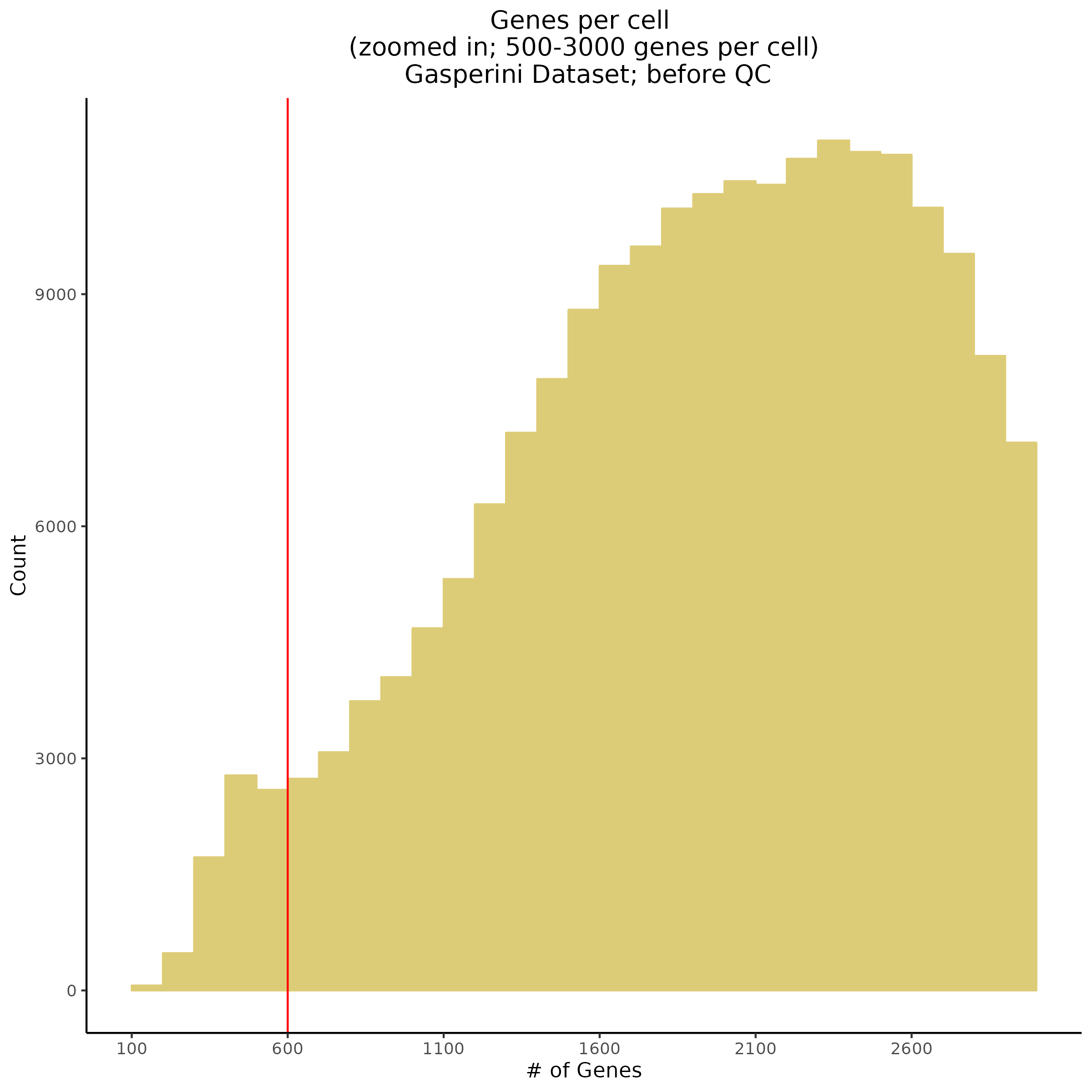
Genes per Cell (uniquely identified genes)
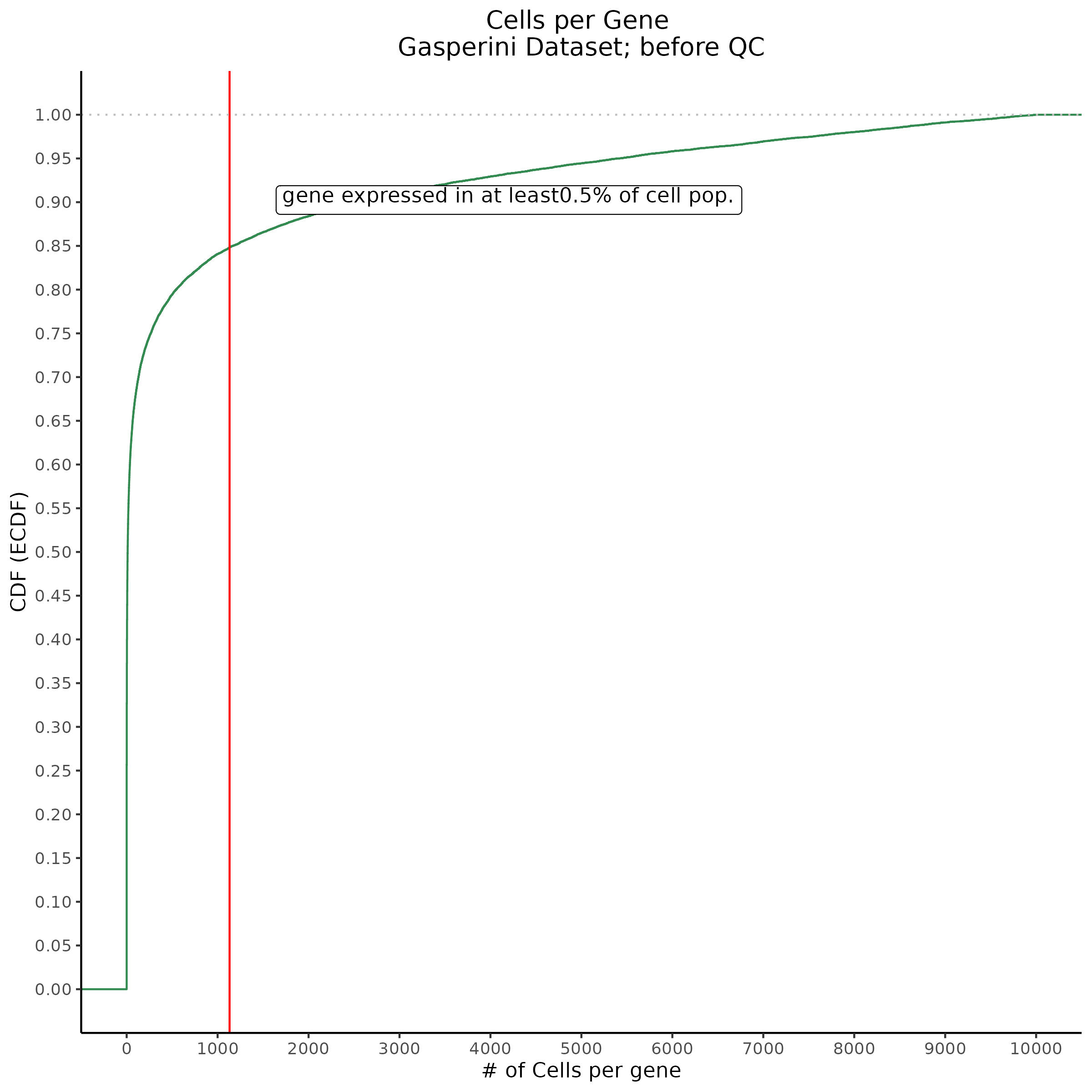
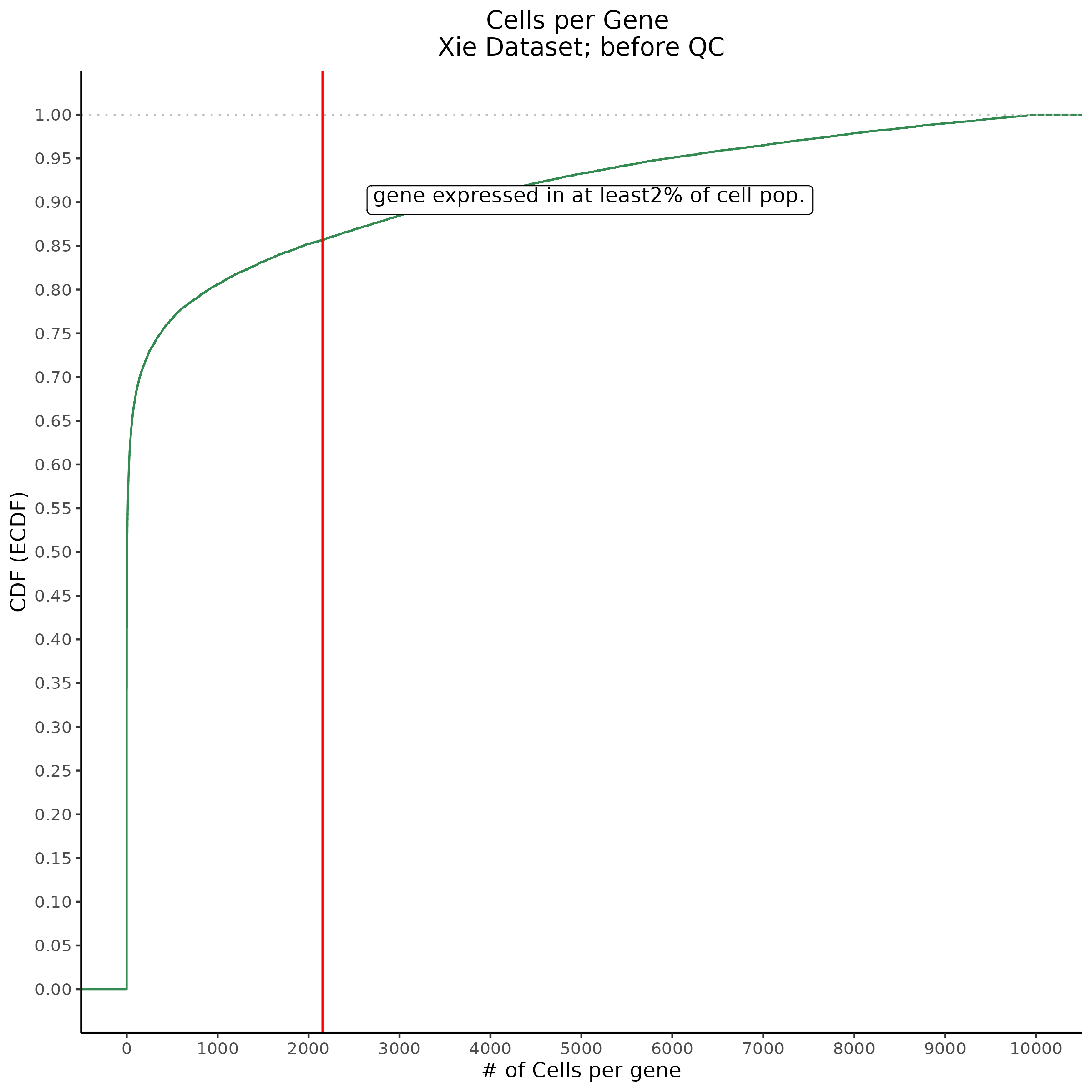
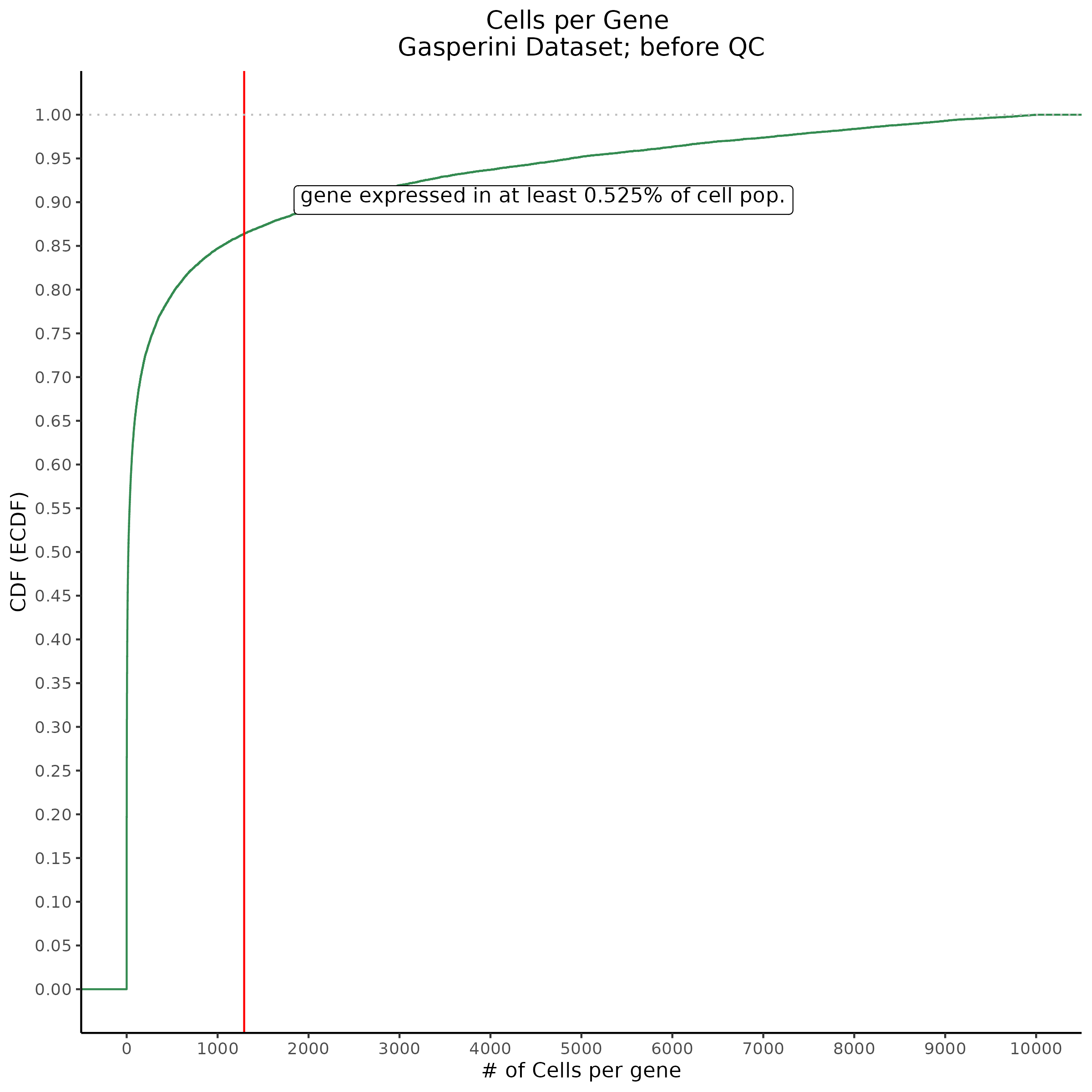
Cells per Gene
This ensures that the gene we test is well expressed in the cell population we are studying (K562). We are using a QC threshold of 0.525% because this was originally defined for this dataset.
“K562 expressed genes were defined as at least one read in 0.525% of cells in the same dataset.” (Gasperini et al. 2019)
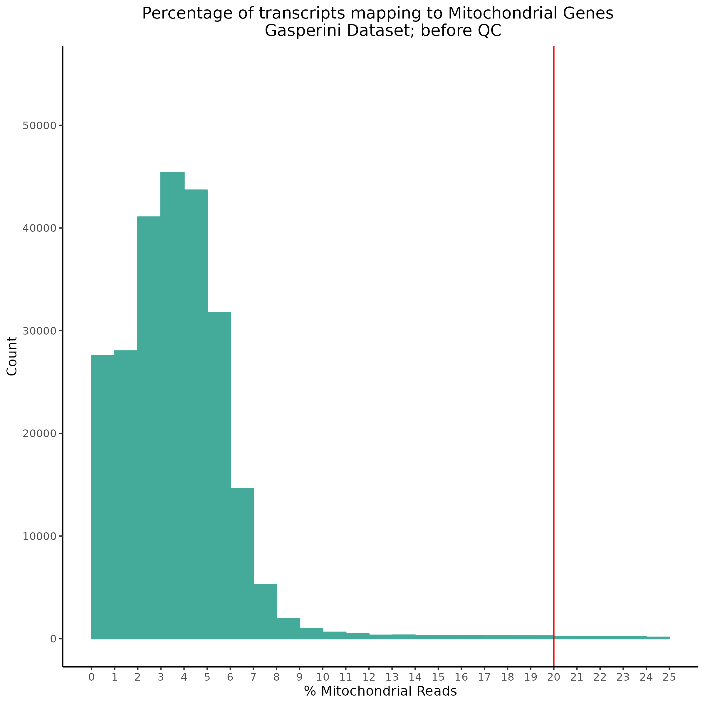
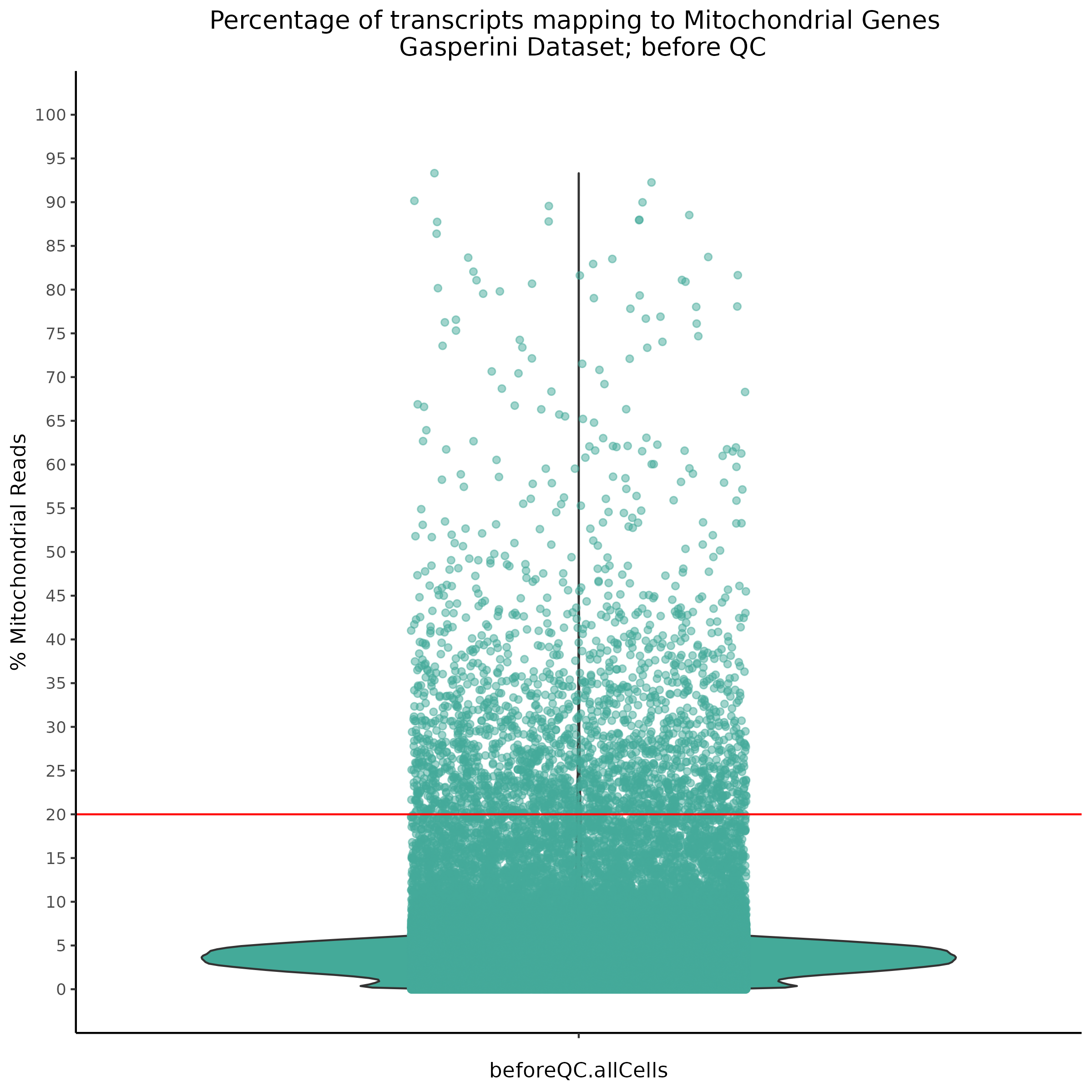
Mito
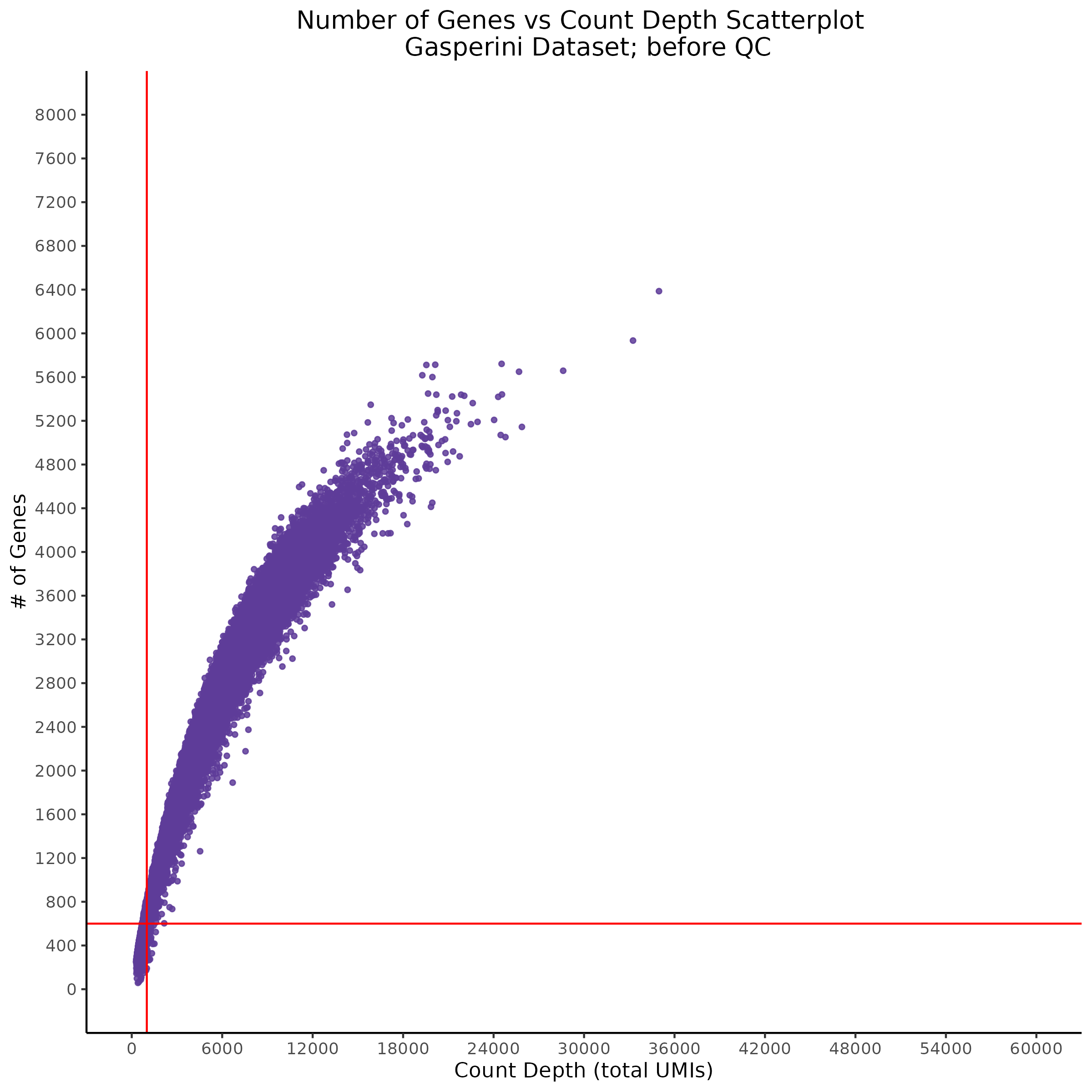
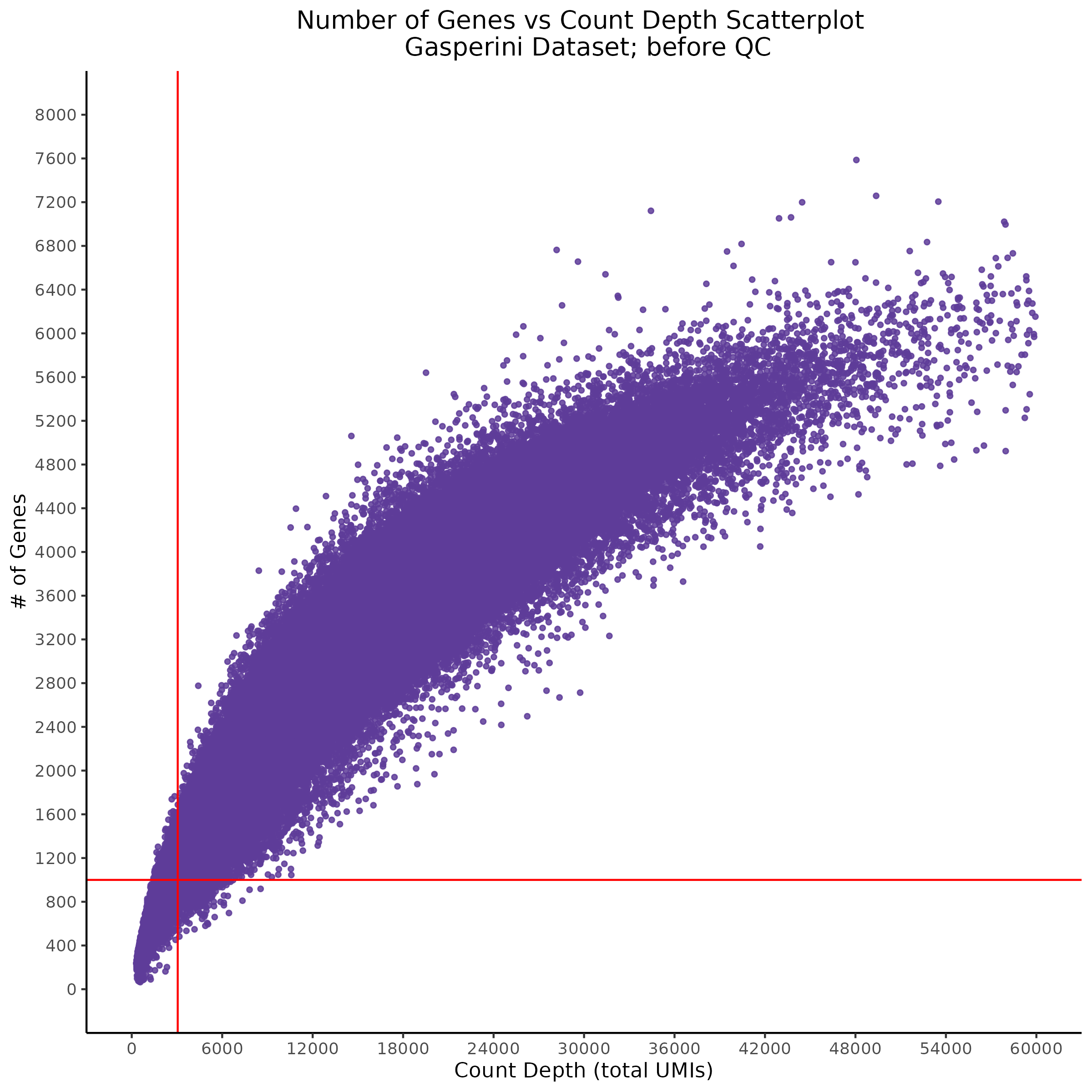
Scatterplot
4/26/23 Morris et al. trans- Signal Rainplots and GRN Plotting
This setion will show the primary results of the Morris trans- analysis.
trans- Signal Rain Plot
![]()
![]()
FDR trans- Signal GRN Plot
![]()
![]()
4/26/23 Xie et al. trans- Signal Rainplots and GRN Plotting
trans- Signal Rain Plot
![]()
![]()
FDR trans- Signal GRN Plot
![]()
![]()
4/12/2023 Xie et al. trans- SCEPTRE Signal Histograms, Cross-Mappable, and NTC Plots
Updated: 4/26/23
Here I will show the results of processing Xie et al trans- sceptre results to show calibration on the NTCs and the % Cross-Mappable Results:
NTC gene-gRNA Pair Histograms (normal/adjusted)
![]()
![]()
% Cross-Mappable
| type | num_fdr_sig |
|---|---|
| SNP | 0.6775956 |
| SNP-Adjusted | 0.3518519 |
3/29/2023 Morris et al. trans- SCEPTRE Signal Cross-Mappable
Updated: 4/26/23
Here I will show the results of processing Morris et al trans- sceptre results to show a table of % Cross-Mappable Results:
% Cross-Mappable
| type | num_fdr_sig |
|---|---|
| SNP | 0.6735537 |
| SNP-Adjusted | 0.5739437 |
3/22/2023 Reverting Processed CellRanger Bam Output
Due to the fast moving nature of single cell research lately some of the older single cell datasets suffer from organizational issues when it related to reprocessing the raw data.
Normally when we browse scRNA seq/CRISPRi pertubation datasets on GEO we will see an option to download the raw data from NCBI SRA repository via something like sratools. For datasets such as Morris et al, Replogle et al, and Xie et al, the rtaw data for the sequencing is availible like so. The general process for downloading and preparing this data would follow the standard sra tools process for unencrypted data. We would download with prefectch and then dump the FASTQ data from the SRA archive. We would then trim reads and perform alignement on the raw FASTQ data with a configured cellranger (configured to the specific RNA-seq/CRISPR perturbation dataset).
But, I have recently encountered a slightly different dataset from Gasperini et al, where the raw data is reported as BAM file. In order to process this data we must first revert it. Why? Becuase actually the BAM is a post-alignment BAM output made by the CellRanger pipeline. In order to recover the original FASTQ files we need to revert this very specific BAM file with the provided Cellranger tool and make sure we do so with the standard metadata. If you were to download and extract the SRA achive the resulting BAM cannot be processed due to missing metadata.
We need to ensure that the version of raw data that we have contains the original metadata encoded into the BAM output by cellranger. To do so, we need to make sure to download the originbal sumbitted data to NCBI not the SRA archive.
1 Download original data [not the usual SRA archive!, key step]
# we will use the standard prefech method for downloading the data
# this command is now modified to include: --type TenX which will download the availible original BAM file with metadata.

/home/nbabushkin/sratoolkit.3.0.0-ubuntu64/bin/prefetch --verbose --verify yes --resume yes --type TenX --option-file sra.txt
Notice that we will skip the extraction step: fastqdump becuase we are not working with SRA archives anymore since the above code will download the original BAM file.
2 Next, we will download the cellranger bam2fastq tool which is used to recover the original FASTQ files from a cellranger BAM output fromt the cellranger github:
wget https://github.com/10XGenomics/bamtofastq/releases/CURRENTRELEASE3 Run the bam2fastq tool to recover original FASTQ input:
/home/nbabushkin/cellranger_bam2fastq/bamtofastq_linux --nthreads=4 at_scale_screen.2A_1_gRNA_AAGTAGCT.grna.bam 2A_1_gRNA_AAGTAGCTThis will in turn recover each of the 4 lanes used the example batch: “2A_1” into the folder: 2A_1_gRNA_AAGTAGCT
bamtofastq_S1_L001_I1_001.fastq.gz
bamtofastq_S1_L001_R2_001.fastq.gz
bamtofastq_S1_L002_R1_001.fastq.gz
bamtofastq_S1_L003_I1_001.fastq.gz
bamtofastq_S1_L003_R2_001.fastq.gz
bamtofastq_S1_L004_R1_001.fastq.gz
bamtofastq_S1_L001_R1_001.fastq.gz
bamtofastq_S1_L002_I1_001.fastq.gz
bamtofastq_S1_L002_R2_001.fastq.gz
bamtofastq_S1_L003_R1_001.fastq.gz
bamtofastq_S1_L004_I1_001.fastq.gz
bamtofastq_S1_L004_R2_001.fastq.gz
We can then re-run a newer (or changed) version of CellRanger count on these FASTQ files, generating another BAM and a set of matrices for this batch. Lastly, we would run cellranger aggregate on all of the counts.
4 Run CellRanger Count (all batches)
5 Run CellRanger Aggregate
3/10/2023 Morris et al. CIS and NTC Analysis using SCEPTRE(s)
This section will explore running SCEPTRE analysis of the already processed Morris data from GEO. This section aims to replicate the original reported results and compare the results of SCEPTRE being run on existing data with respect to NTC calibration, cis signals, and distribution of the pairs made by Morris et al originally.
Summary of Significant cis- gene-gRNA pair Results
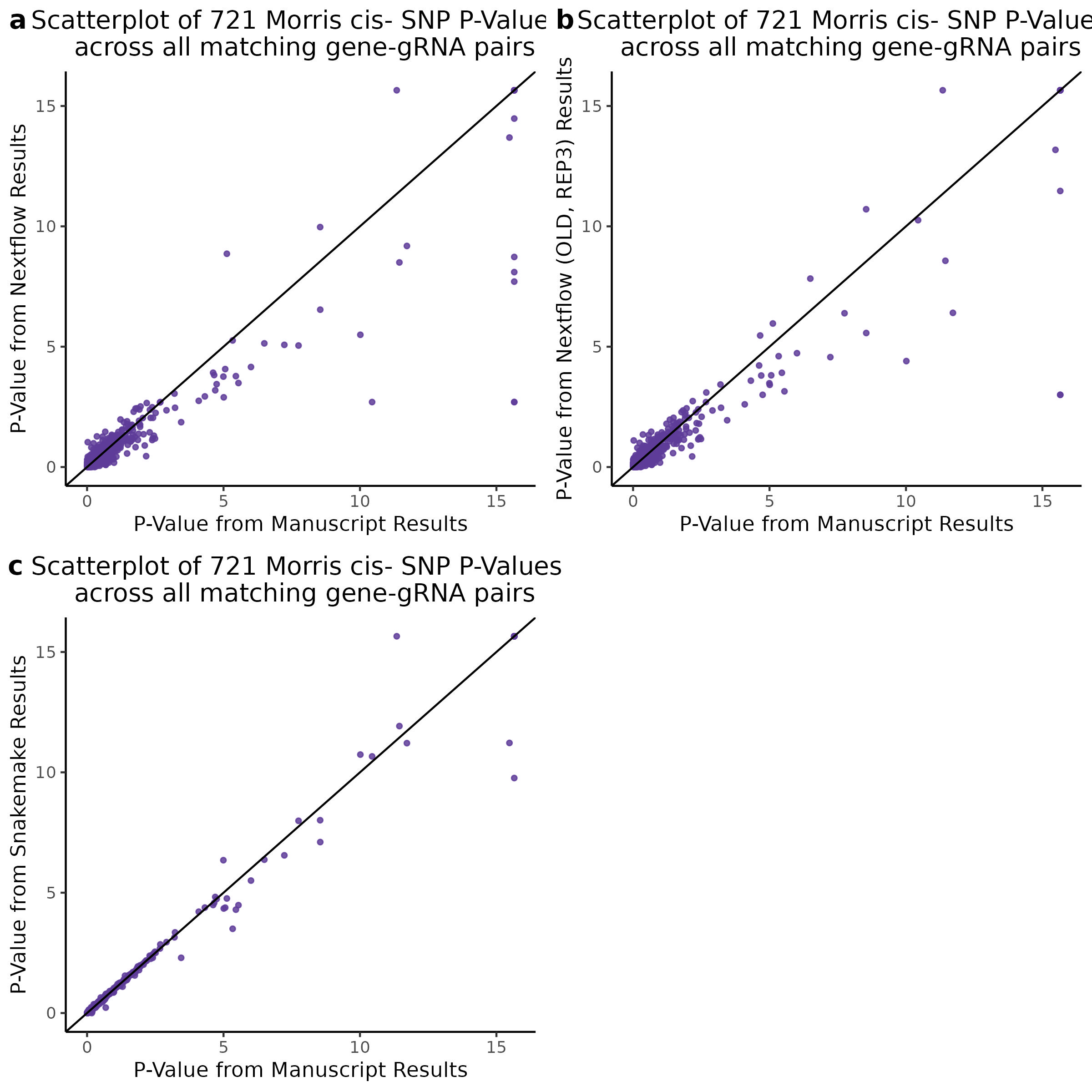
| comparisons | fdr_sig | bonferroni_sig |
|---|---|---|
| original SCEPTRE results | 54 | 36 |
| nextflow SCEPTRE | 50 | 24 |
| snakemake retroSCEPTRE | 55 | 35 |
Morris cis- gene-gRNA Pair P-Value SCEPTRE Comparison
Morris NTC P-Value SCEPTRE Comparison
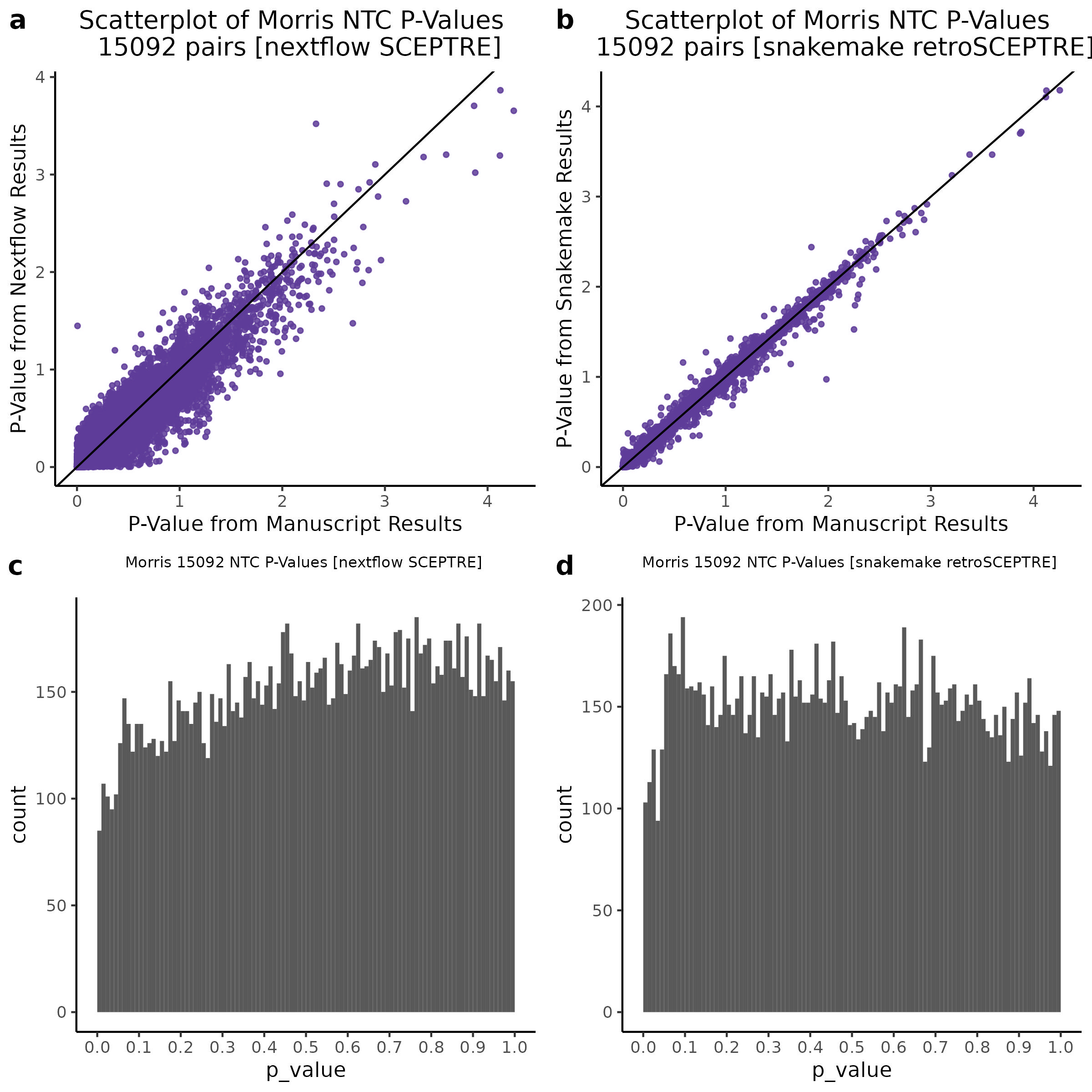
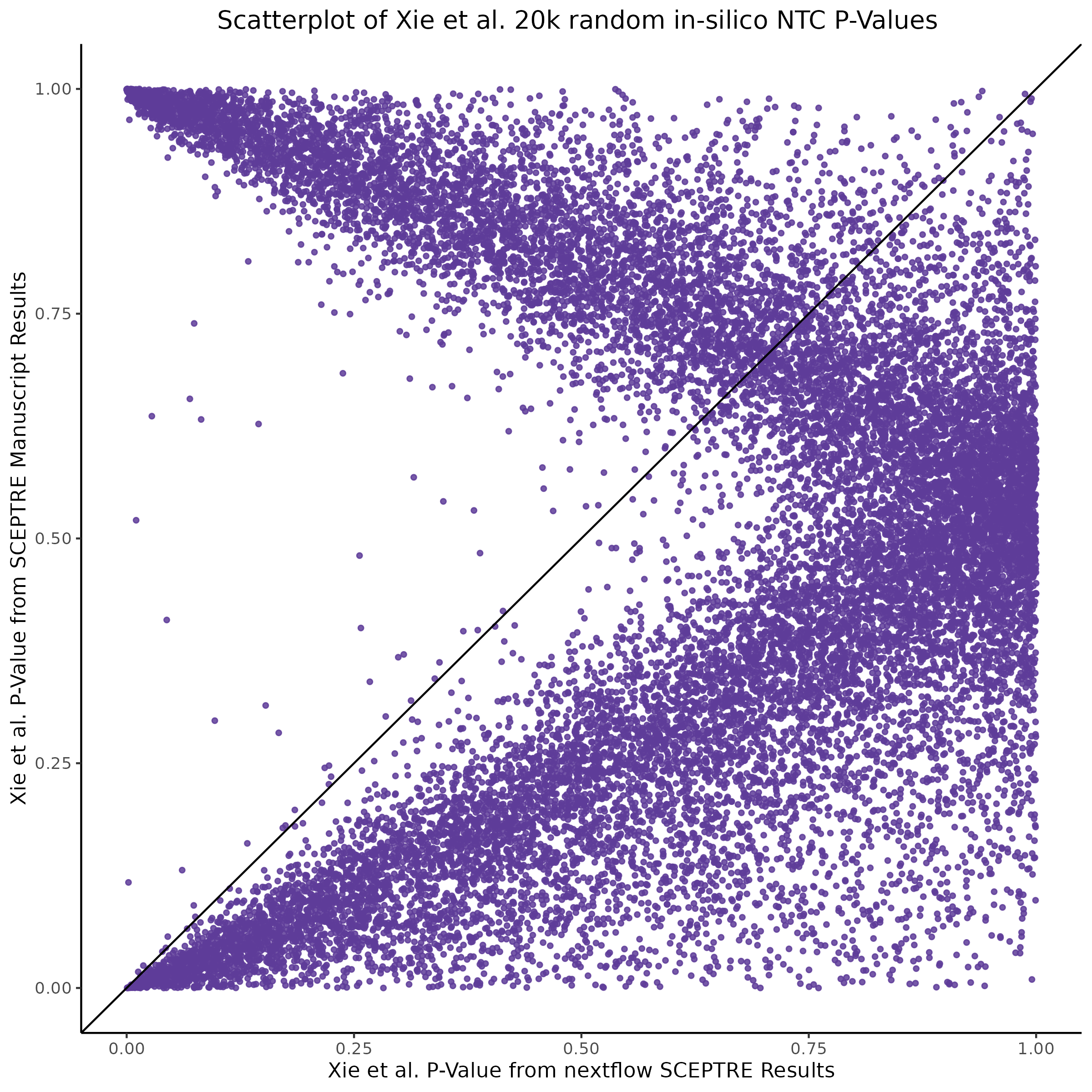
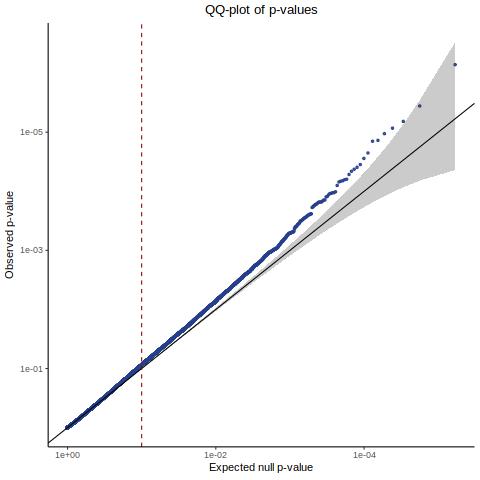
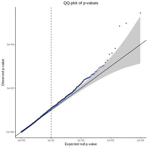
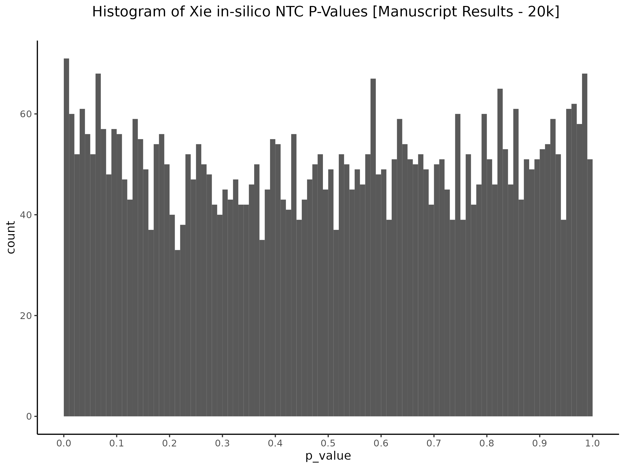
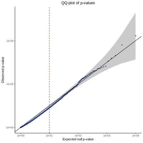
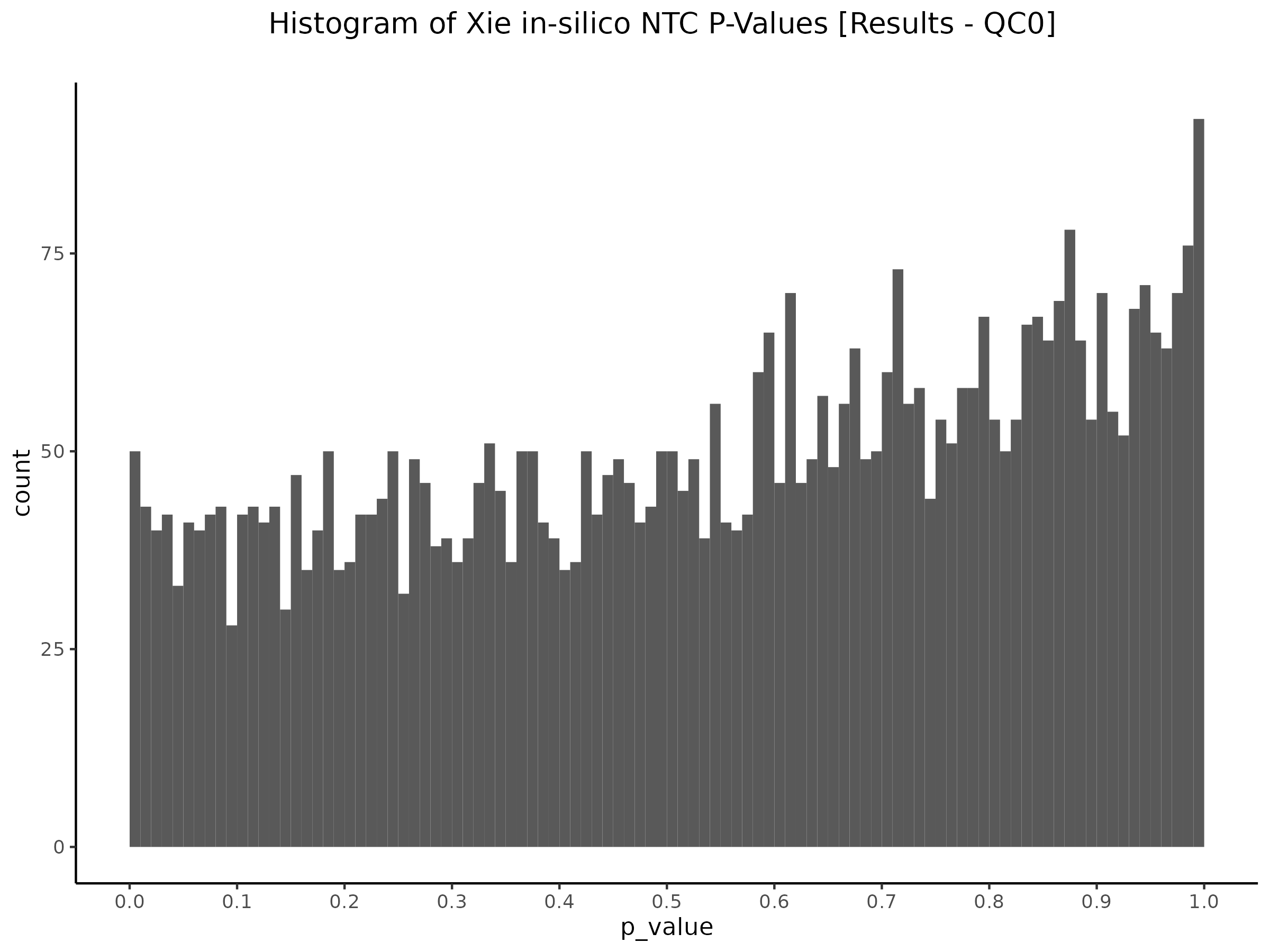
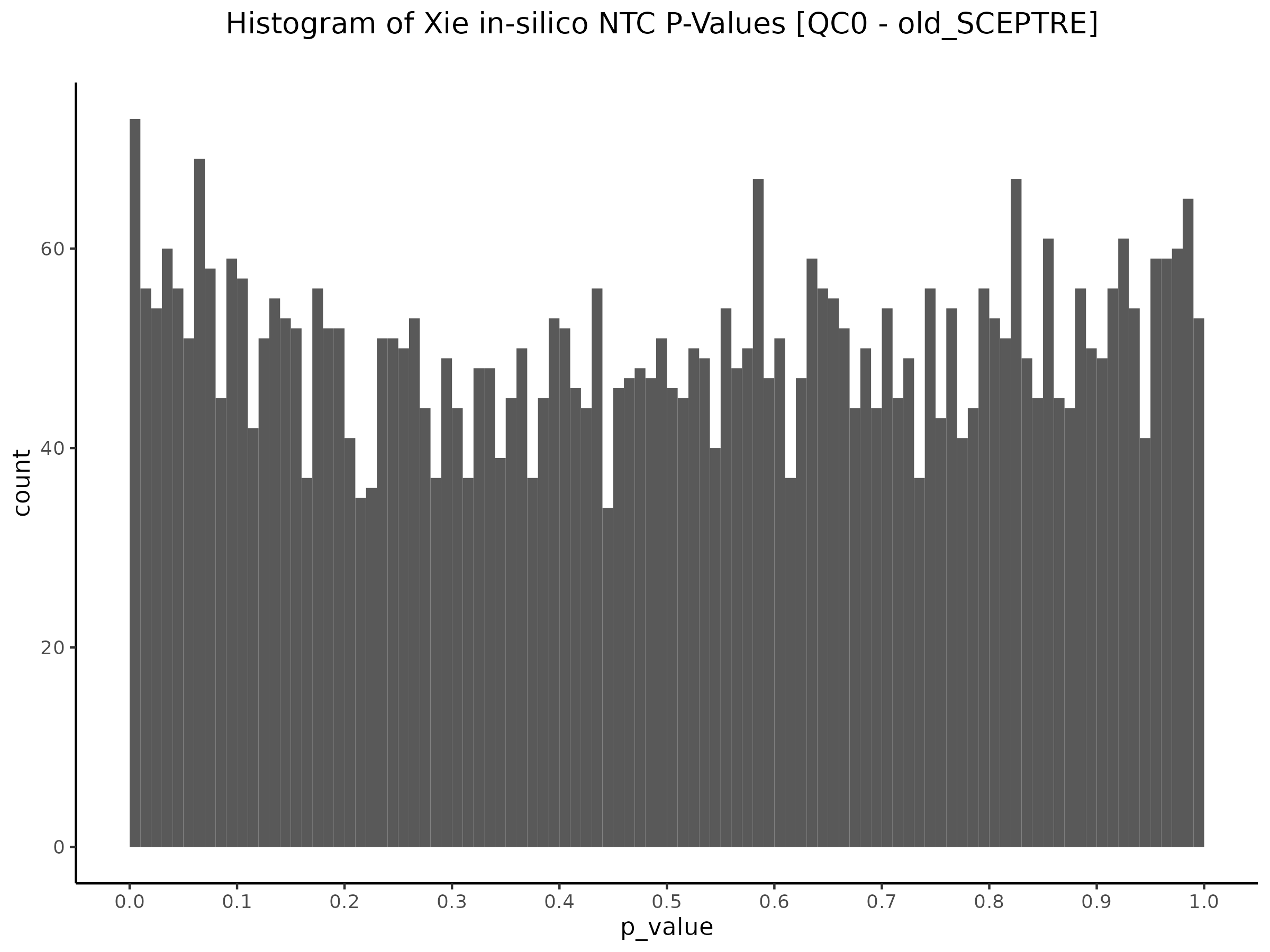
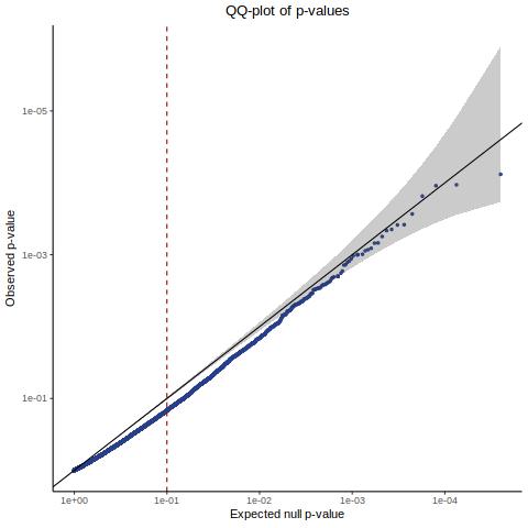
3/2/2023 Xie et al. NTC Analysis using SCEPTRE(s)
This section will explore running SCEPTRE analysis of scRNAseq data from Xie et al., with an emphasis on the p values and distribution of SCEPTRE results for the in silico non-targetting controls used in the original manuscript. To this end, this section will show that for a 5,000 gene-gRNA pair subset of the total 84,500 NTC pairs, SCEPTRE has differing results conditional on the SCEPTRE method used. In summary, we believe we are seeing a skew in the distribution of p values associated with the non targetting controls when the newer, version 1.0.0 of SCEPTRE package is used alongside its nextflow pipeline. In contrast, the original results do now show this skew for the 5,000 gene gRNA pair subset that was selected for evaluation tests. When analyzing these pairs using an in house SCEPTRE-snakemake package built upon the original manuscript SCPETRE package, we see that the p values produced are roughly equivalent by Pearson R correlation accross all 5,000 p values to those p values produced in the original manuscript analysis. Notably this SCEPTRE version produces p values for the in silico NTCs that are not skewed, as seen in panel C.
print('loading historic insilico results: ')
hist_results = read_fst('/project/xuanyao/nikita/SCEPTRE/data/Xie_2019/Xie_manuscript_downloaded_process/results_BOXdl/all_results_annotated.fst') %>% as.data.table()
hist_insilico_ntc_results = hist_results %>% filter(type == 'negative_control') # pair_str is already there

print('loading QC results')
# our manu re-run: QC0: Yx ~ Xx + Cx  ====> yx_xx_cx
qc0_check_5kNTC = readRDS('/scratch/midway3/nbabushkin/Xie_QC0_SCEPTRE_CHECK3/sceptre_results.rds') # 5k results here
qc0_check_5kNTC = qc0_check_5kNTC %>% rowwise %>% mutate(pair_str = paste0(grna_group,'+',gene_id)) %>% ungroup()

qc0_retro_sceptre = read_fst('/scratch/midway3/nbabushkin/Xie_retroSCEPTRE/results/all_results.fst')
qc0_retro_sceptre = qc0_retro_sceptre %>% rowwise %>% mutate(pair_str = paste0(gRNA_id,'+',gene_id)) %>% ungroup()

qc0_retro_sceptre_snakemake = read_fst('/scratch/midway3/nbabushkin/Xie_QC0_SCEPTRE2_test2/results/all_results.fst')
qc0_retro_sceptre_snakemake = qc0_retro_sceptre_snakemake %>% rowwise %>% mutate(pair_str = paste0(gRNA_id,'+',gene_id)) %>% ungroup()

print('comparing 5k NTC results...')
qc0_w_historic_5k = qc0_check_5kNTC %>% left_join(hist_insilico_ntc_results %>% select(pair_str, hist_p_value = p_value, gene_name), by = 'pair_str')
qc0_w_historic_5kretro = qc0_retro_sceptre %>% select(gene_id, gRNA_id, p_value,z_value,  pair_str) %>% left_join(hist_insilico_ntc_results %>% select(pair_str, hist_p_value = p_value, gene_name), by = 'pair_str')
qc0_w_historic_5kretrosnakemake = qc0_retro_sceptre_snakemake %>% select(gene_id, gRNA_id, p_value,z_value,  pair_str) %>% left_join(hist_insilico_ntc_results %>% select(pair_str, hist_p_value = p_value, gene_name), by = 'pair_str')

check1 = cor(qc0_w_historic_5k$p_value, qc0_w_historic_5k$hist_p_value) # [1] -0.2058252 3-3-3
check2 = cor(qc0_w_historic_5kretro$p_value, qc0_w_historic_5kretro$hist_p_value) # [1] 0.9999586 now! 3!
check3 = cor(qc0_w_historic_5kretrosnakemake$p_value, qc0_w_historic_5kretrosnakemake$hist_p_value) # 0.977 [1] ...

print('(based on a random sample of 5k in silico NTCs made by manuscript, total: 84.5K NTCs)')
print(paste0('[QC0 calibration; old SCEPTRE v0.1.0] QC0 Pearson R based on historical, reported results: ', check2))
print(paste0('[QC0 calibration; nextflow SCEPTRE v1.0.0] QC0 Pearson R based on historical, reported results: ', check1))
print(paste0('[QC0 calibration; retro SCEPTRE (aka snakemake SCEPTRE)] QC0 Pearson R based on historical, reported results: ', check3))
This code outputs the follow pearson R correlation results:
[1] "[QC0 calibration; old SCEPTRE v0.1.0] QC0 Pearson R based on historical, reported results: 0.999958613825321"
[1] "[QC0 calibration; nextflow SCEPTRE v1.0.0] QC0 Pearson R based on historical, reported results: -0.20592926049342"
[1] "[QC0 calibration; retro SCEPTRE (aka snakemake SCEPTRE)] QC0 Pearson R based on historical, reported results: 0.977527051289071"
From this we can expect the nextflow SCEPTRE results to be quite different, while the snakemake SCEPTRE / retroSCEPTRE results seem to be right on top and possibly differing only due to a randomness mismatch due to the extremely high Pearson R accross the raw p values output by .
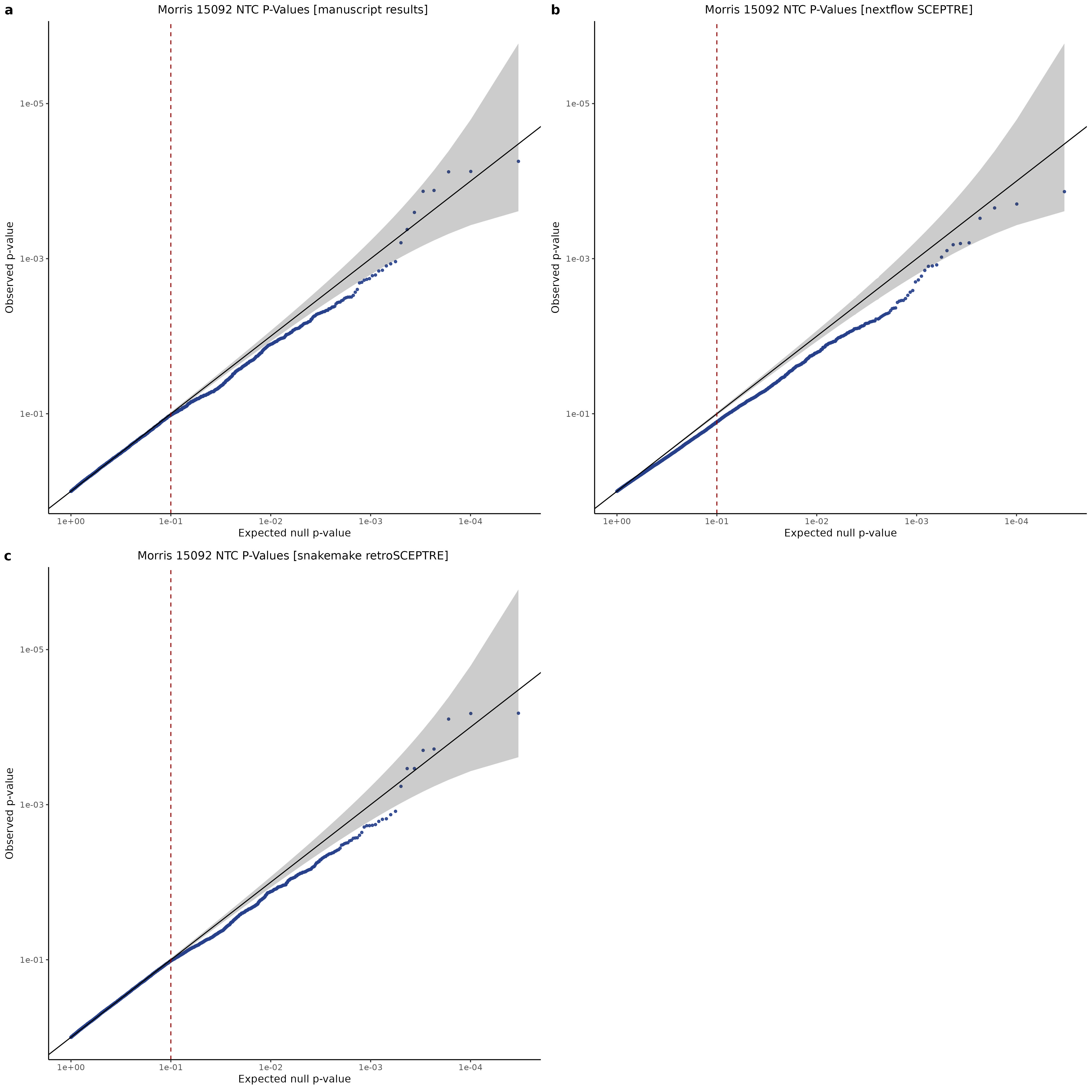
To further really explore how the p values are distributed we can make QQ plots and histograms of the raw p values produced by each method: 1) original results 2) nextflow SCEPTRE 1.0.0 package 3) retroSCEPTRE/snakemake SCEPTRE.
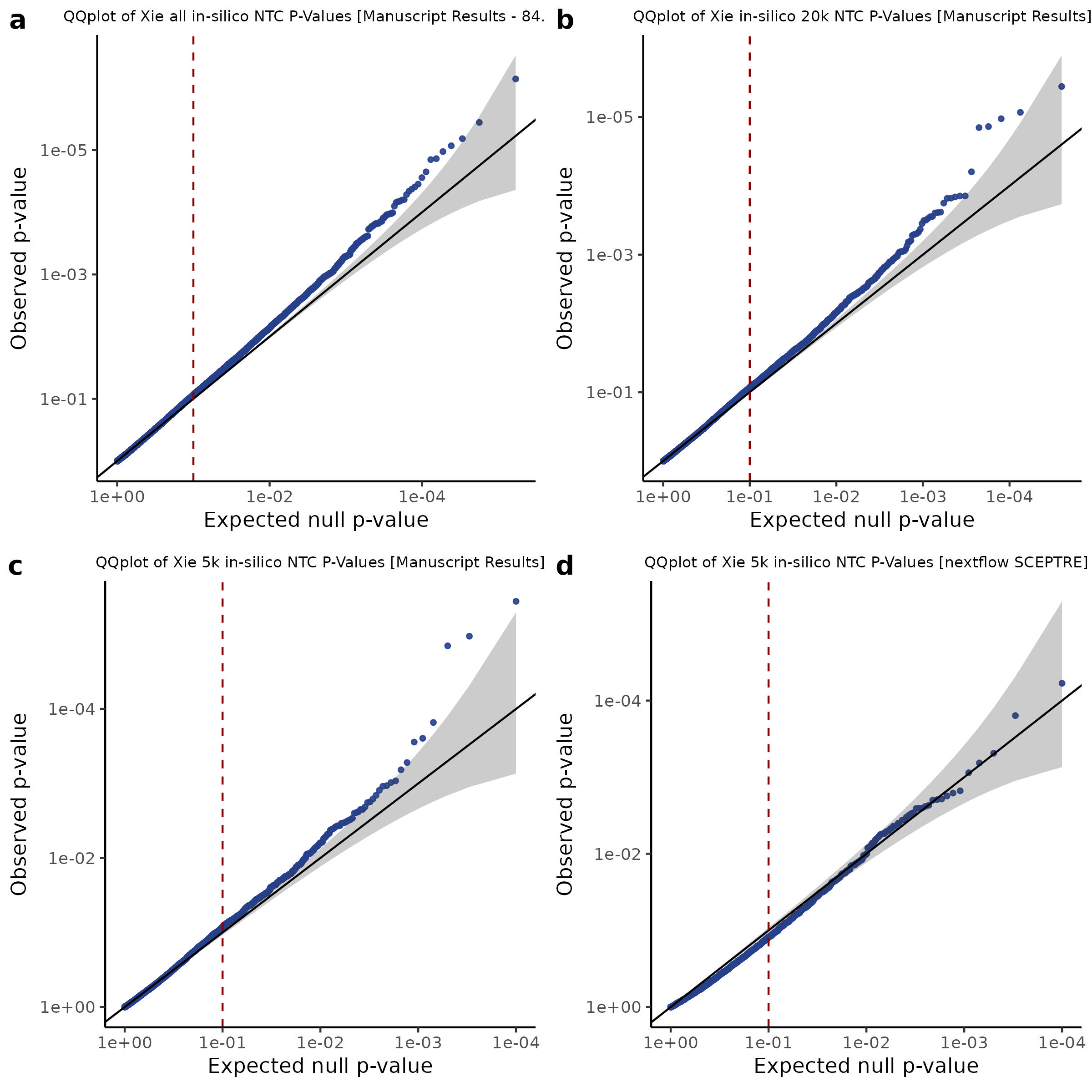
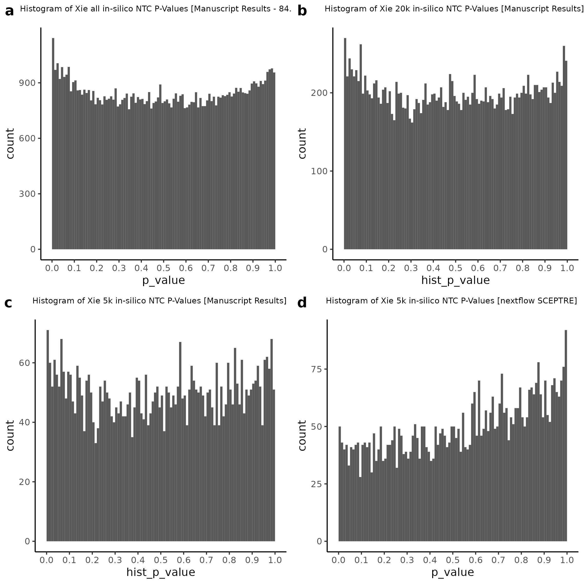
Then we can also plot scatter plots too see another pattern evident only in the nextflow or v1.0.0 SCEPTRE.
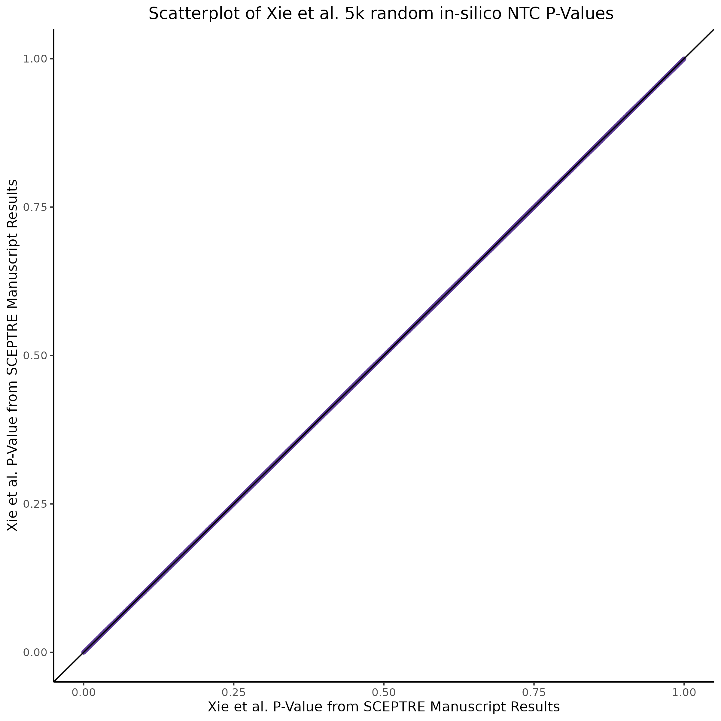
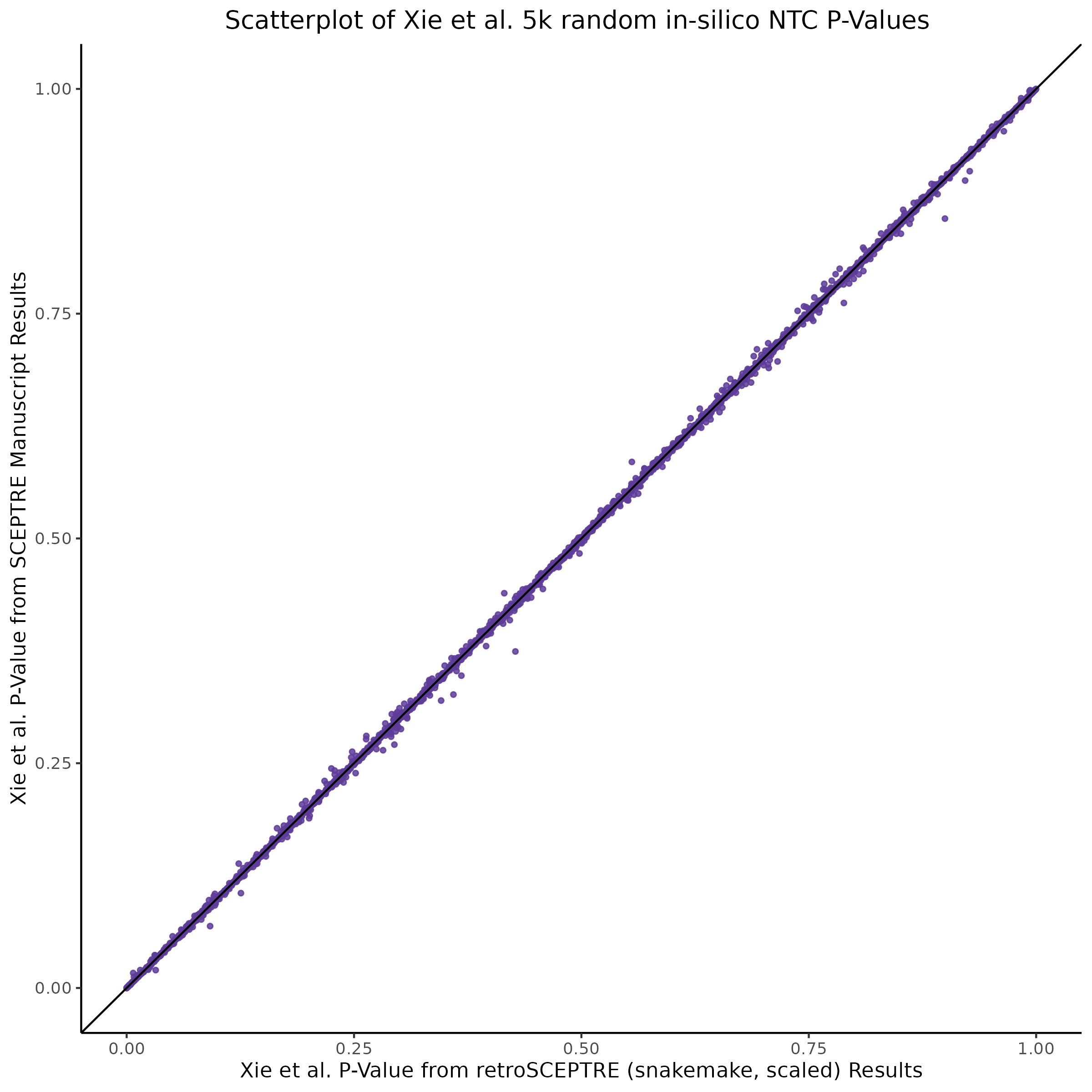
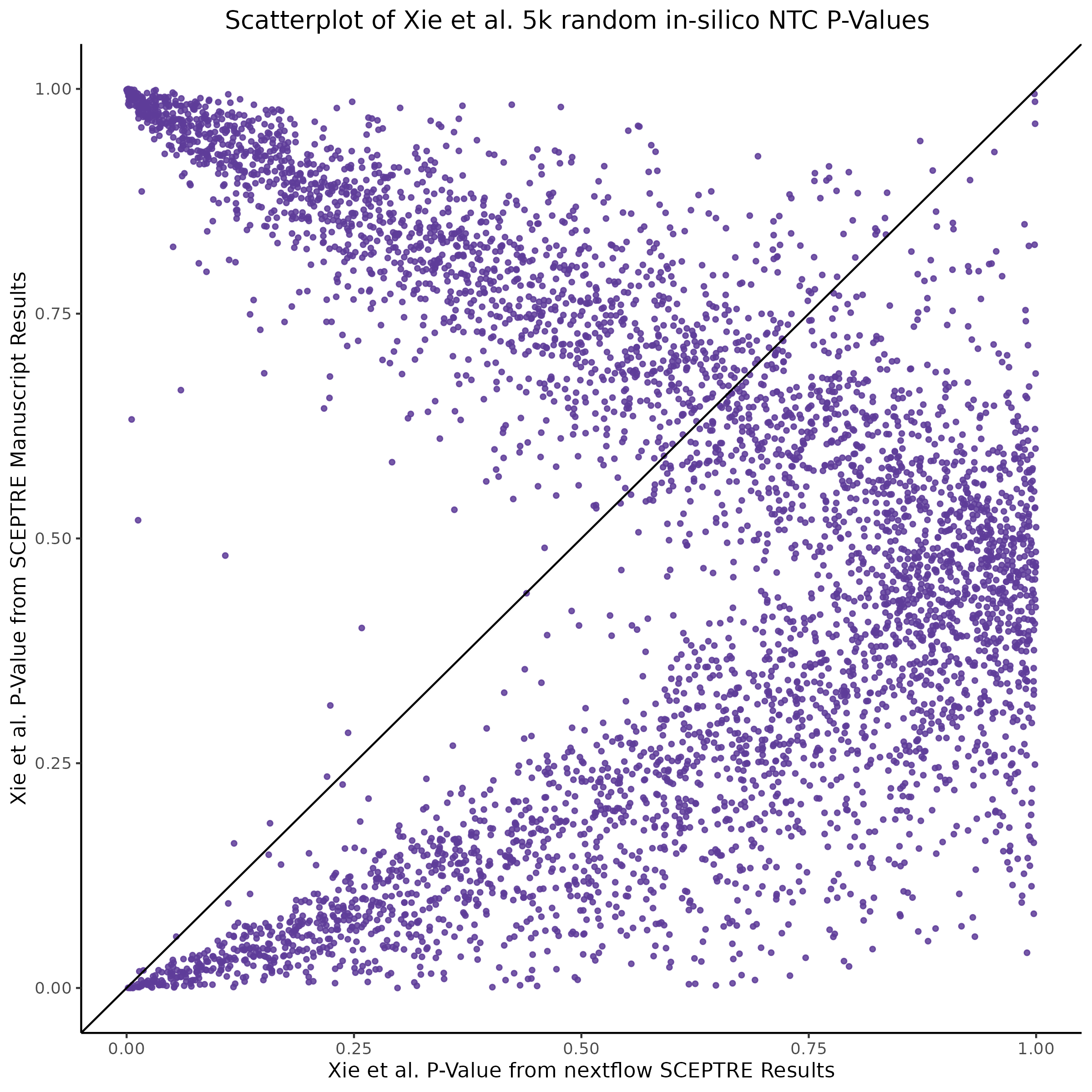
This is accentuated if we look at 20k in silico NTCs using the nextflow SCEPTRE.
2/15/2023 Xie et al. QC NTC Plots Continued.
This section will show the results of various different QC configurations aimed at recalculating manuscript results, and to compare the processed matrices input into SCEPTRE against our own re-processed with CellRanger matrices and SCEPTRE input.
QC Historic - Histogram/QQplot
This shows the original manuscript results for all 84.5K in silico NTC pairs. Here the results are read directly from those reported in the mansuscript and re-plotted.
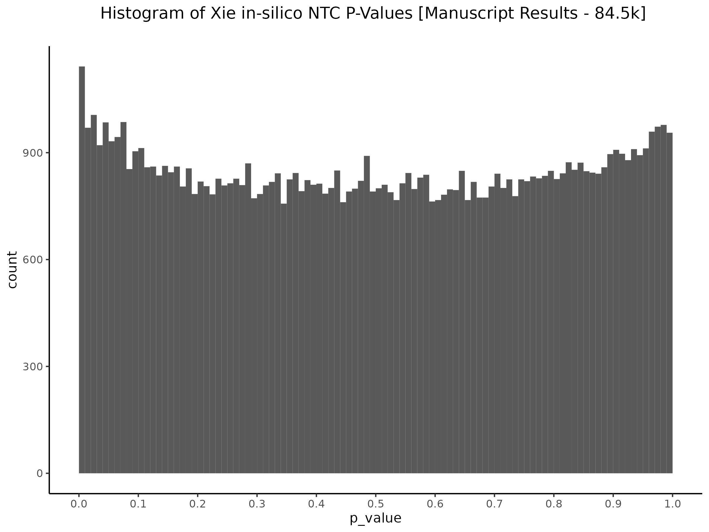
This is essentially Figure 3 from the manuscript.
QC Historic 5k subset - Histogram/QQplot
This is the original manuscript NTC results subset to a set of 5k NTCs that we will later compare against (both by visual-plotting and pearson R of p values).
This is roughly the same as above since this is a subset of those shown in the first, control qq plot.
QC0 [Y(GEO) ~ X(GEO) + C(GEO)] - Histogram/QQplot
This is the modern rendition of the manuscipt results. Specifically, here we are utilizing the Nextflow SCEPTRE pipeline to evaluate the original manuscirpt pairs. Here we are using a gene expression and gRNA pertubation matrix from the manuscipt (GEO-sourced+manuscript code), including their covariates. The goal here is to use all inputs that are identical to the original inputs used in the manuscript. The expectation is that the p values for the subset of 5k in silico NTCs will be the same. We expect the qqplot to also be similar for these pairs due to the exactedness of the input.
QC0 “old” SCEPTRE [Y(GEO) ~ X(GEO) + C(GEO)] - Histogram/QQplot
Here we utilize the old SCEPTRE version.

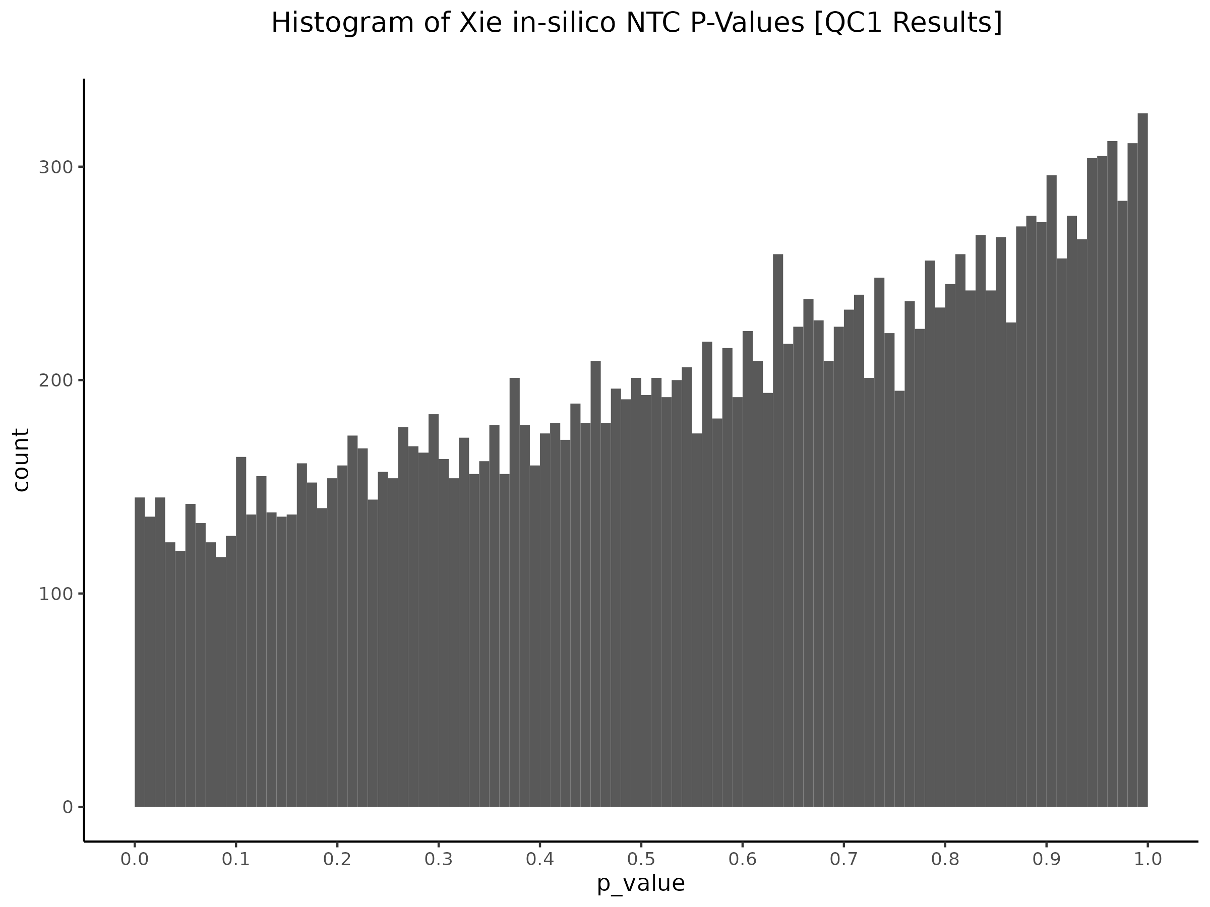
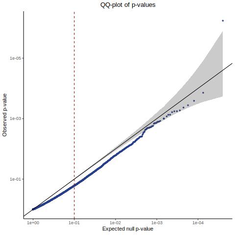
QC1 [Y(ours) ~ X(GEO) + C(GEO)] - Histogram/QQplot
Here we are now changing the gene expression input matrix to be sourced from our re-processing (CellRanger count+aggr output). But we are still using the original covaraites and gRNA matrix.
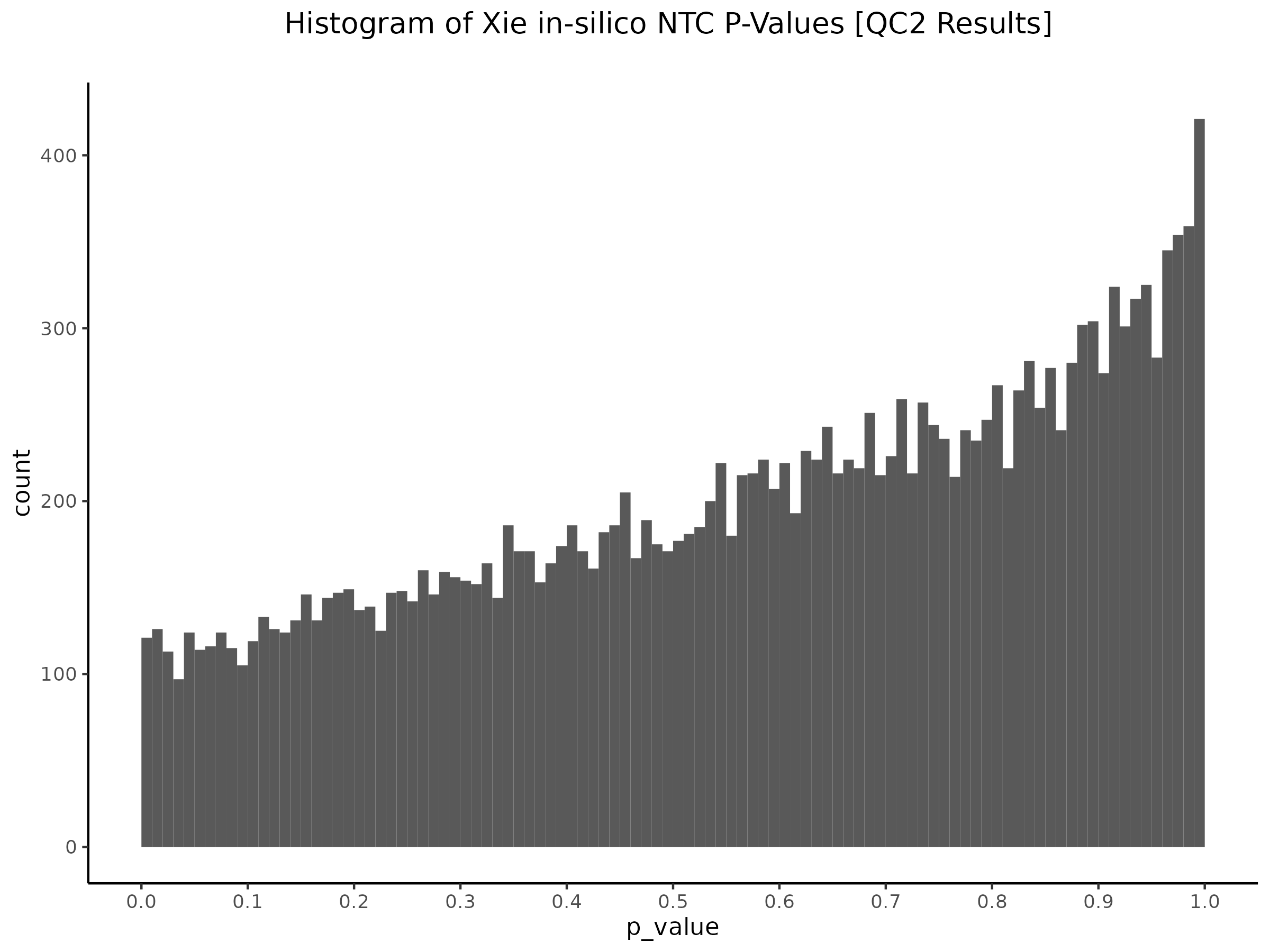
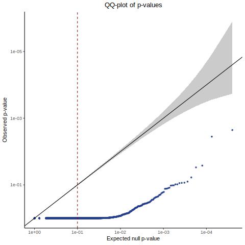
QC2 [Y(GEO) ~ X(ours) + C(GEO)] - Histogram/QQplot
Here we are now using our own gRNA input matrix to be sourced from our re-processing (CellRanger count+aggr output).
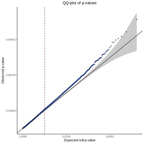
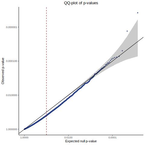
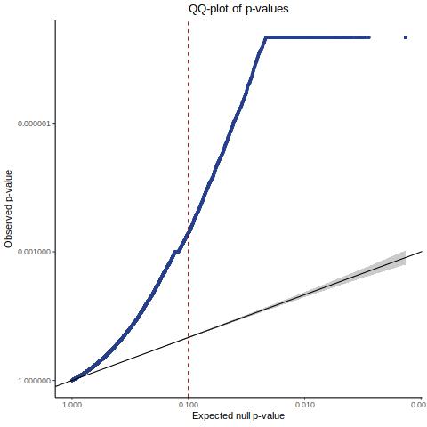
QC3 [Y(GEO) ~ X(GEO) + C(ours)] - Histogram/QQplot
Here we are now using our covariates but we are sourcing the matrices from the manuscript input.
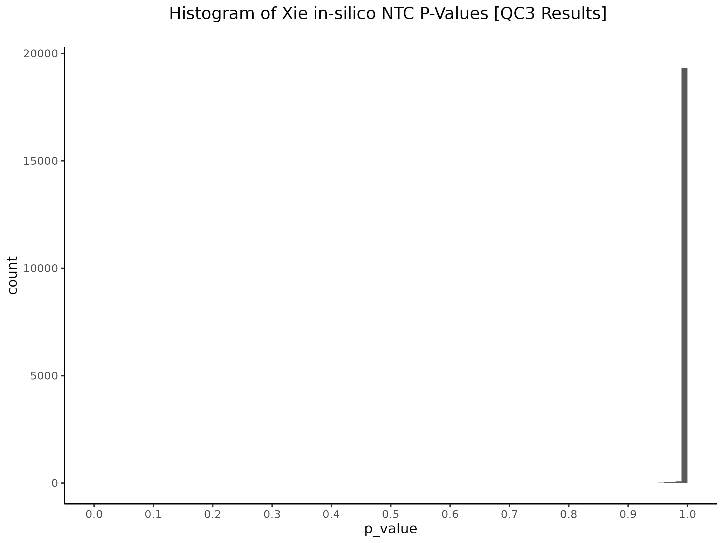
Xie et al. NTC Plots (Based on SCEPTRE Manuscript)
In this section we are trying explore the NTC pairs in Xie et al. dataset used in the SCEPTRE manuscript. In the manuscript the authors run SCEPTRE on the Xie et al. dataset, analyzing candidate CIS pairs and in silico NTC pairs, as well as bulk validations pairs. By re-running the entire analysis we can take a look at the effects of grouping guides together and the usage of in silico controls as NTC, versus the traditional method of designing non-targeting sgRNAs within the CRISPRi experiment.
We start by re-plotting Fig. 3 from the manuscript:
This is strongly similar to Figure 3 shown in the manuscript paper.
Next we can plot our results of the same in silico gene-gRNA NTC pairs:
Lastly we can plot just sgRNA-NTC-1 and sgRNA-NTC-3 NTC guides, paired with all availible genes:
Intro Network Plotting of Morris et al. Trans- signal Results
The general idea is visualize Trans- signal in a dataset as a network. As an test, we will make network plots using the signal from Morris et al Trans- results using igraph and network libraries in R.
# read in results, extract gRNAs
results = read_fst('/project/xuanyao/nikita/SCEPTRE/results/Morris_cis_and_trans_analysis/Morris_trans_SCEPTRE_results_10_13/Morris_SCEPTRE_results_short.fst') %>% as.data.table()
gRNAs = results %>% pull(gRNA_id) %>% unique()

# select FDR sig. results, create edge table
# here 'gRNA'-'gene' pairs > populate 'source'-'target' columns in table
# importance = -log10(results_fdr$bh_adjusted_pvalue) could be used to set width of connections later
results_fdr = results %>% filter(bh_rejected)
links = data.table(source = results_fdr$gRNA_id, target = results_fdr$gene_id)

# make vertices list from edge-link table source-target columns
vertices <- unique(unlist(c(links$source,links$target)))
# constuct color vector + node table using vertices list
netnodes = data.table(name = vertices) %>% mutate(colors = ifelse(name %in% gRNAs, sample(colors, replace = TRUE), '#888888'), )

# init. network w/ link table + node table
net <- graph_from_data_frame(d=links, vertices=netnodes, directed=F)

# save + output plot w/ colors
color_vector <- netnodes$colors
png(file=paste0(out_dir, '/node.png'), width=5000, height=5000,  res=300)  # width=1000, height=1000,  res=300
plot(net, edge.arrow.size=.3, vertex.size=3, vertex.color=color_vector, vertex.label.cex=0.8, vertex.label = ifelse(V(net)$name %in% gRNAs, V(net)$name, NA))
title(main = 'Network Plot using FDR gRNA-gene Pairs as Source-Target', cex.main = 2, sub = NULL, xlab = NULL, ylab = NULL)
legend( "bottomright", legend = c('gRNA', 'Gene'), pt.bg  = c('#332288','#888888' ), pch    = 21, cex    = 3.3, bty    = "n", title  = "Node Type:"  )
dev.off()
Here is the plot result. The grey nodes represent genes found in FDR signficant gRNA-gene pairs, while nodes in a random (colorblind-safe) color represent gRNAs.
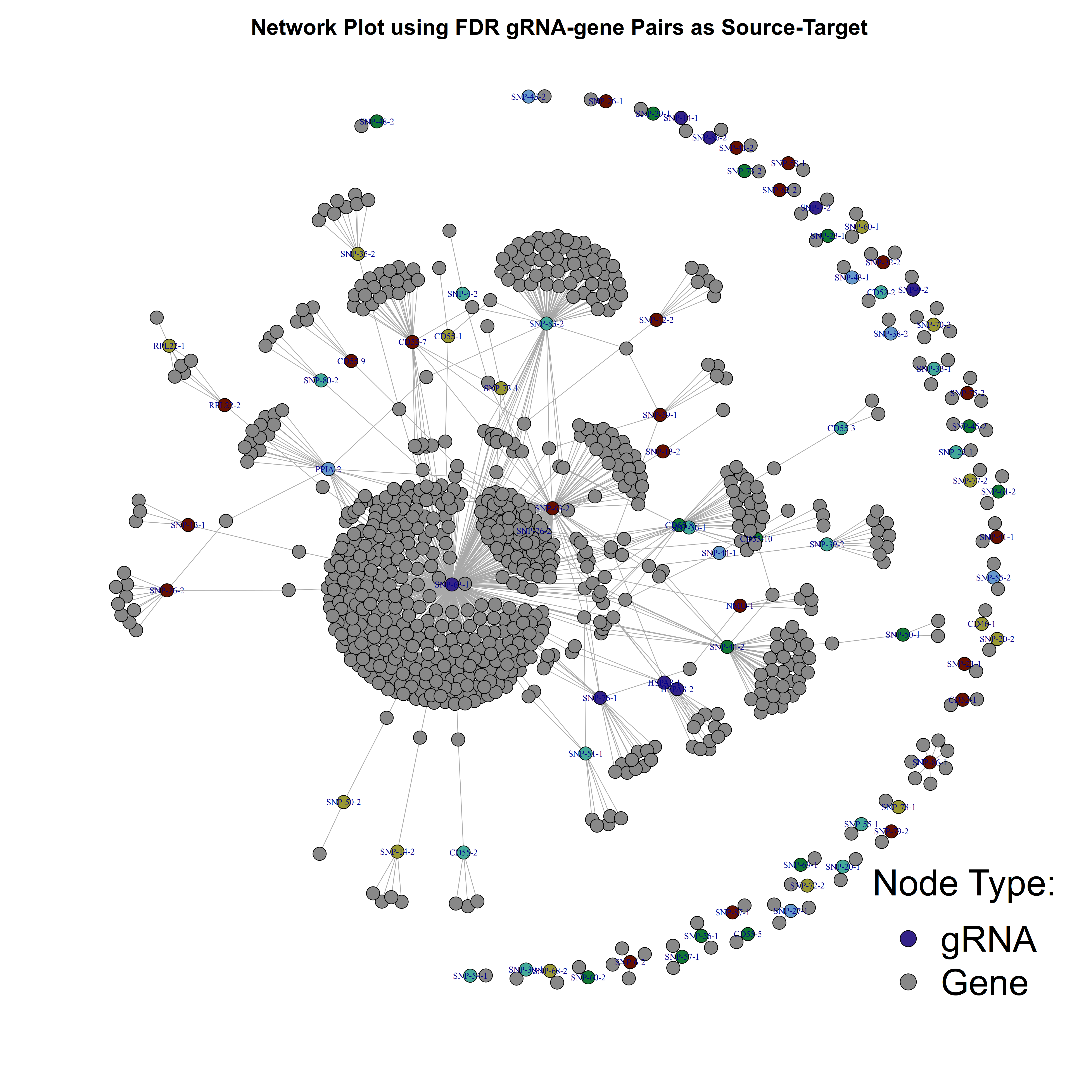
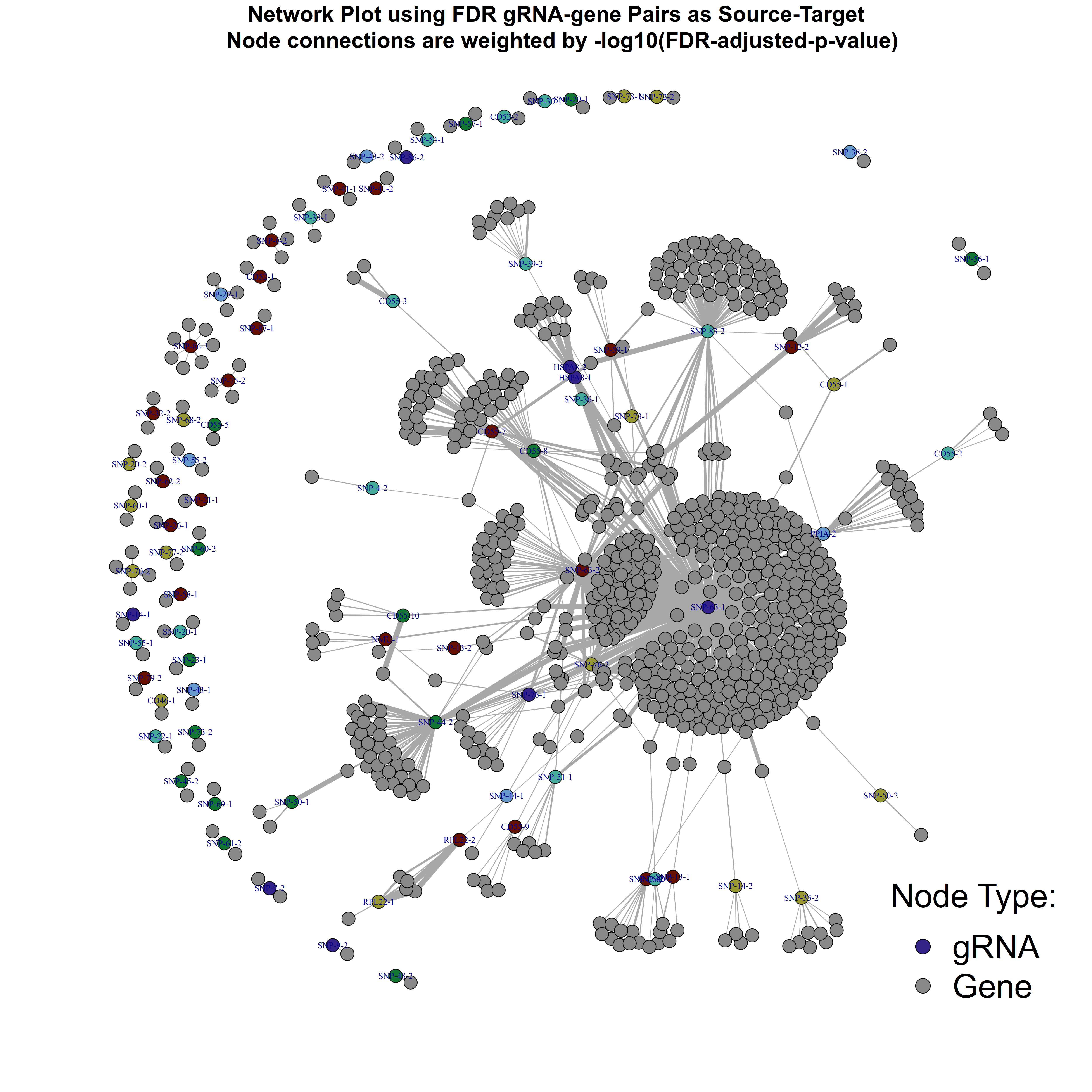
One way we can modify this further is to use the adjusted p-values as weights in order to show the connection strengh between a given gRNA and gene pair within our plot.
color_vector <- netnodes$colors
png(file=paste0(out_dir, '/node2.png'), width=5000, height=5000,  res=300)  # width=1000, height=1000,  res=300
# we add edge.width=E(net)$importance*.7 to scale the node links using the importance column
plot(net, edge.arrow.size=.3, vertex.size=3, edge.width=E(net)$importance*.7, vertex.color=color_vector, vertex.label.cex=0.8, vertex.label = ifelse(V(net2)$name %in% gRNAs, V(net2)$name, NA),)
title(main = 'Network Plot using FDR gRNA-gene Pairs as Source-Target \n Node connections are weighted by -log10(FDR-adjusted-p-value)', cex.main = 2, sub = NULL, xlab = NULL, ylab = NULL)
legend( "bottomright", legend = c('gRNA', 'Gene'), pt.bg  = c('#332288','#888888' ), pch    = 21, cex    = 3, bty    = "n", title  = "Node Type:"  )
dev.off()
Final plot for FDR sig. Trans- gRNA-gene pairs in Morris et al.
Xie et al. Dataset QC and SCEPTRE Preprocessing
In order to run SCEPTRE we need to first perform QC, generate covariate matrices, and place the matrices into an ondisc H5 multimodal matrix, which is then the primary input to SCETPRE. We also need to generate gene-gRNA pairs based on information after QC is performed.
QC
Below is an outline of the general QC parameters used
- Min. cells per gene: 0.0525 % (of cells)
- Min. genes per cell: 700
- Min. count depth: 1250 (min. total UMIs per cell)
- Max sgRNA UMIs per cell: 15,000
- Min. cells per sgRNA: 50
- Min. sgRNA threshold: 5 UMIs (used to generate the binary matrix indicating presence/lack of sgRNA in a given cell)
Covariate Matrix:
We will also generate a initial covariate matrix based on the cDNA/GDO data. But it is important to note that this matrix is only used to create the final covariate matrix, which is stored within the multimodal ondisc H5 object.
The following covariates are necessary for SCEPTRE:
- gene_p_mito
- lg_gene_n_nonzero
- lg_gene_n_umis
- lg_gRNA_n_nonzero
- lg_gRNA_n_umis
- batch number
Two important things must be noted: these are based on filtered outputs, from CellRanger, specific to each cell barcode and these utilize information from QC. Notably the percent mitochondrial reads must be derived based on the reference used during QC. The number of sgRNAs that are unique or non-zero, is also based on the thresholded gRNA matrix. For example, we would not count a sgRNA in a cell with a count of 4 becuase this is below our threshold of 5, and the binary matrix would not indicate a presence of that sgRNA, so the covariate matrix must not count this sgRNA towards that cell’s total unique sgRNA count.
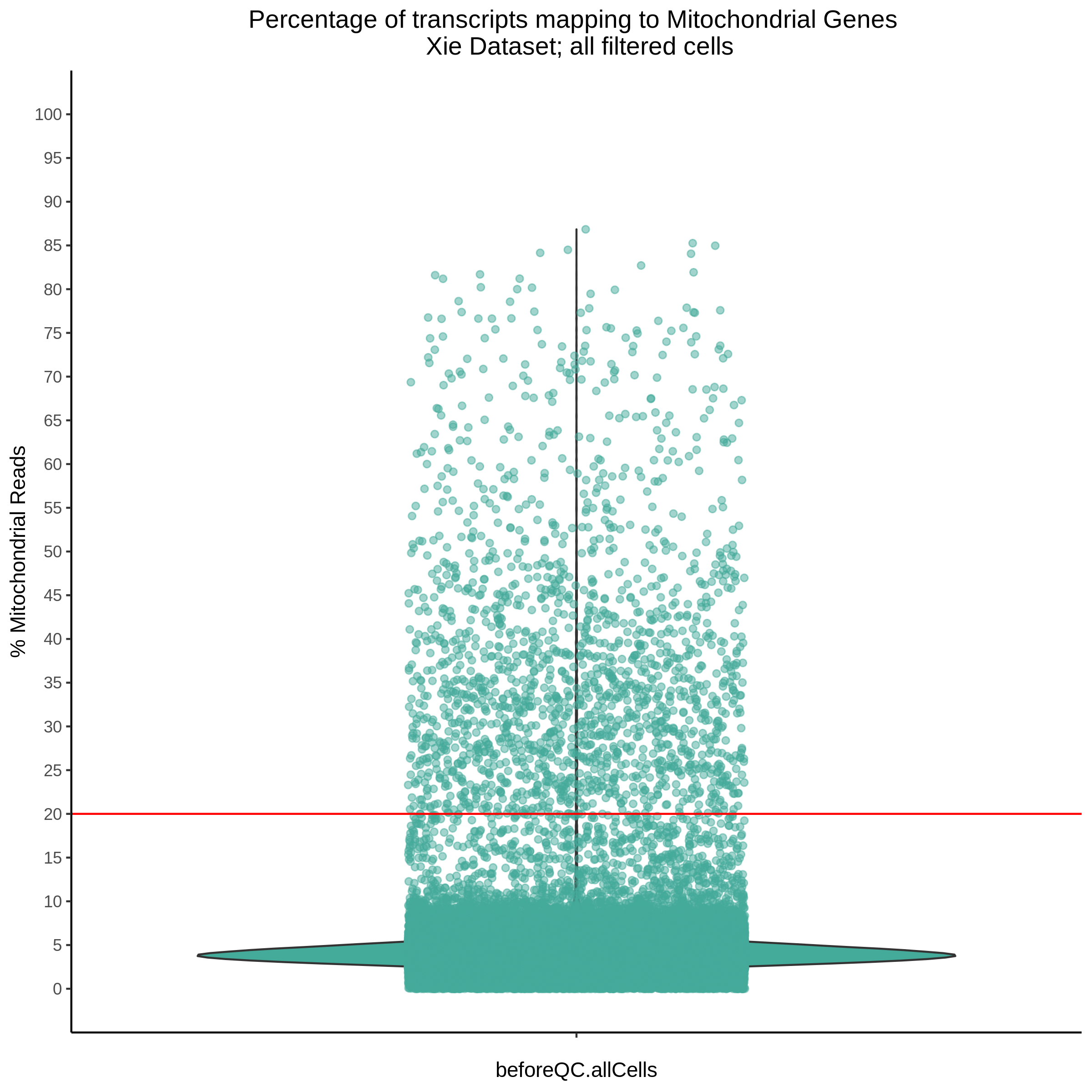
QC Plot-Results before QC:
These QC plots are meant to show the dataset after it has been filtered by Cellranger, but before we apply the QCs above.
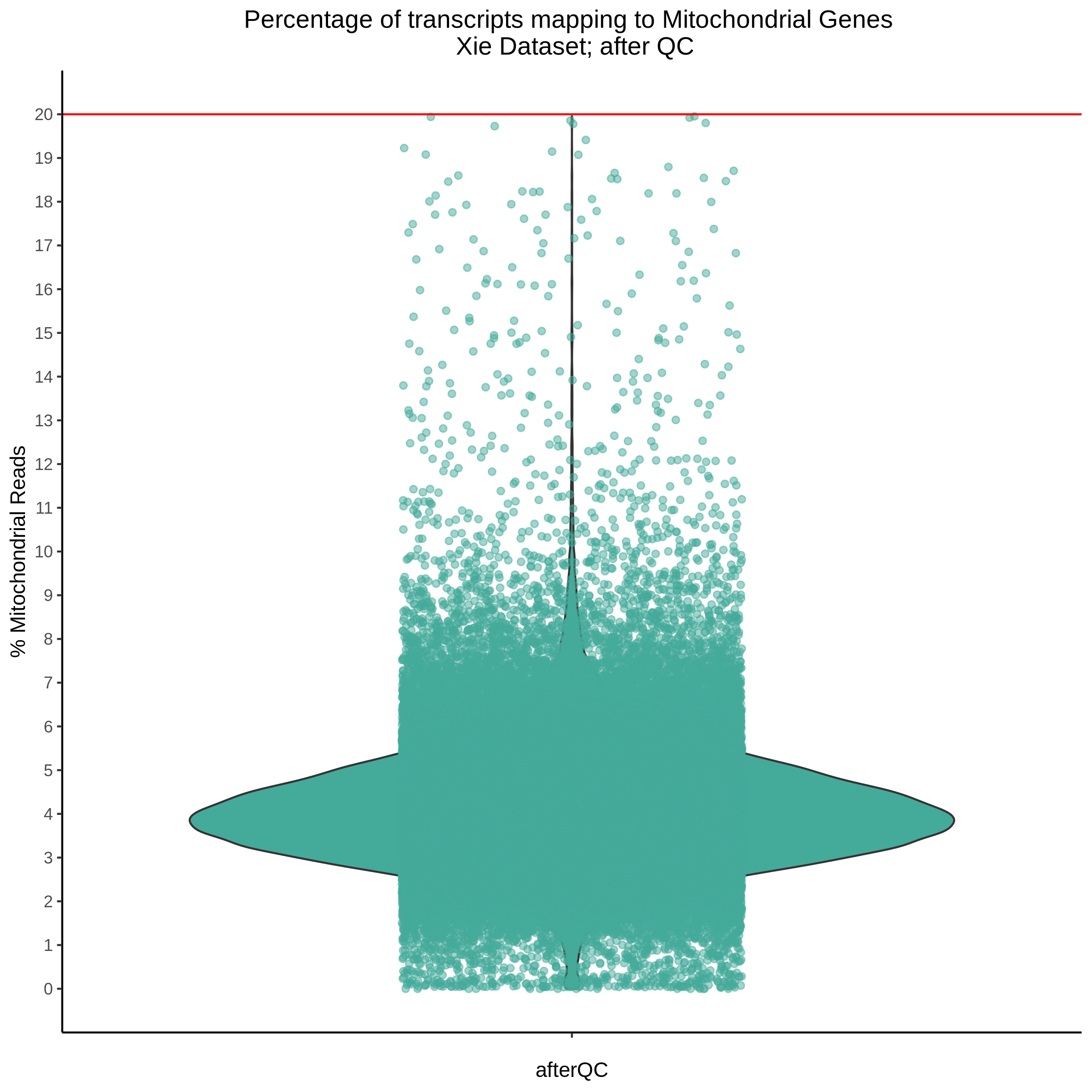
- Plot showing the percent of mitochondrial reads in all cells before QC. A red line is placed at 20%, the threshold for mitochondrial contaminated cells.
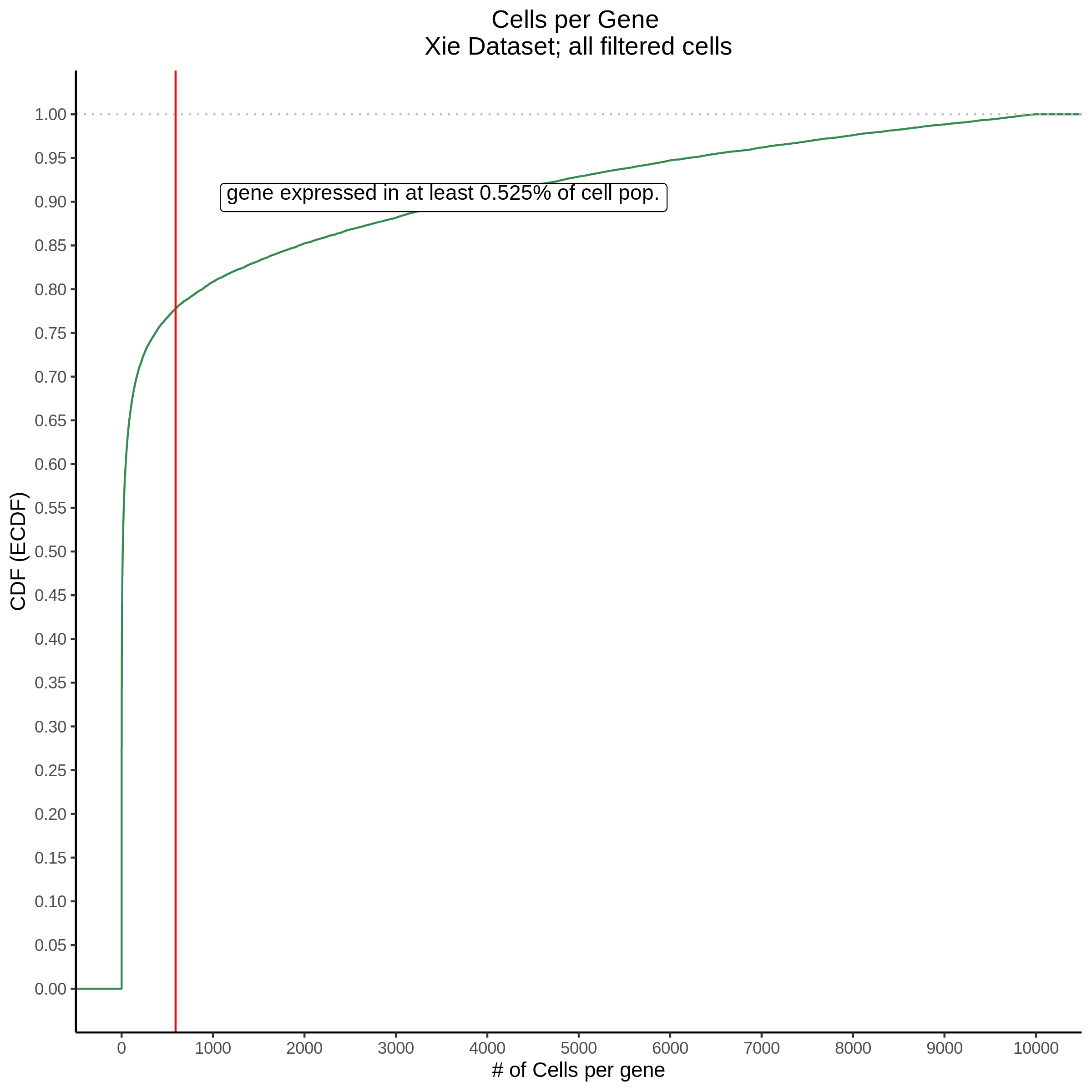
- Plot showing cells per gene in CDF plot, a red line is placed at .0525% of total cells.
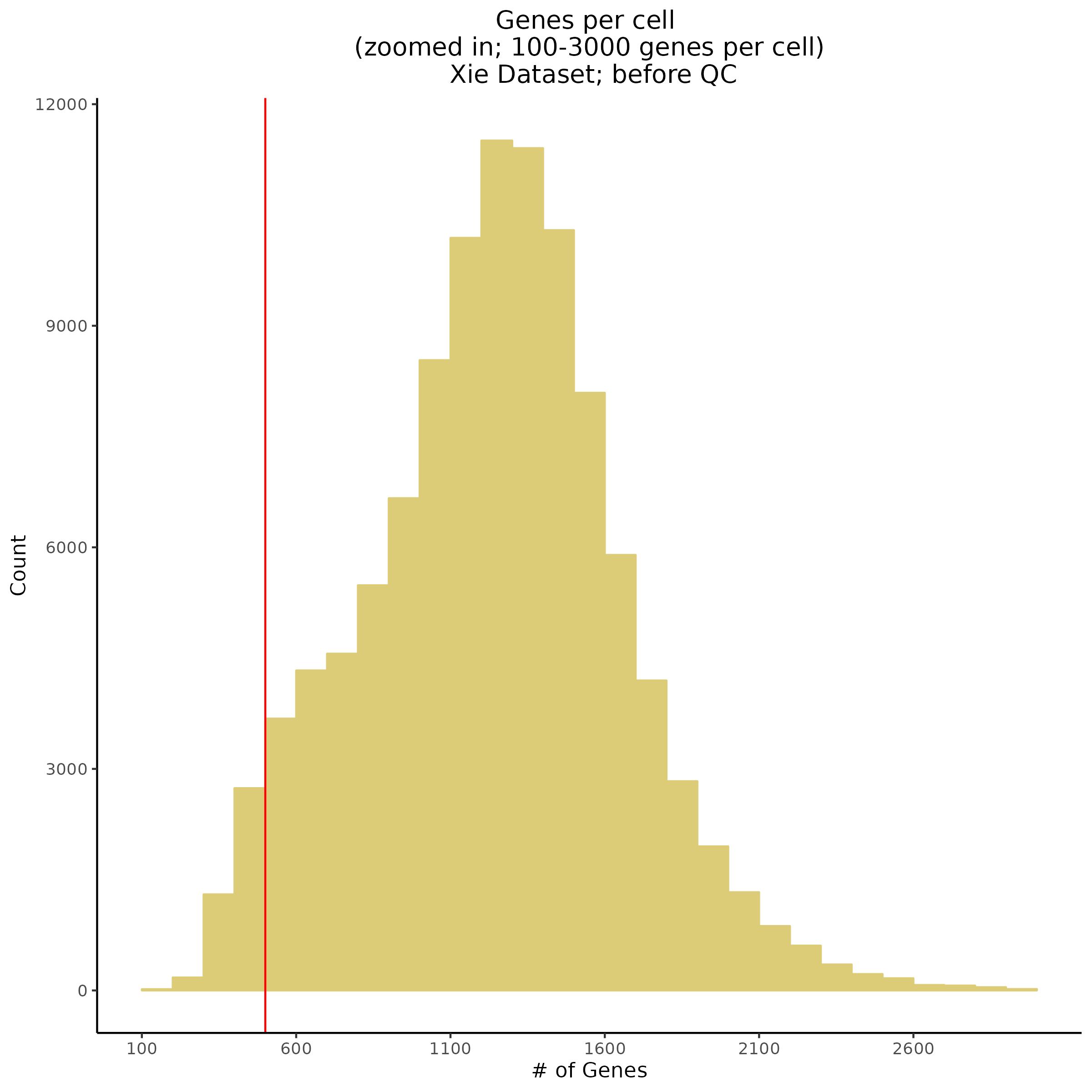
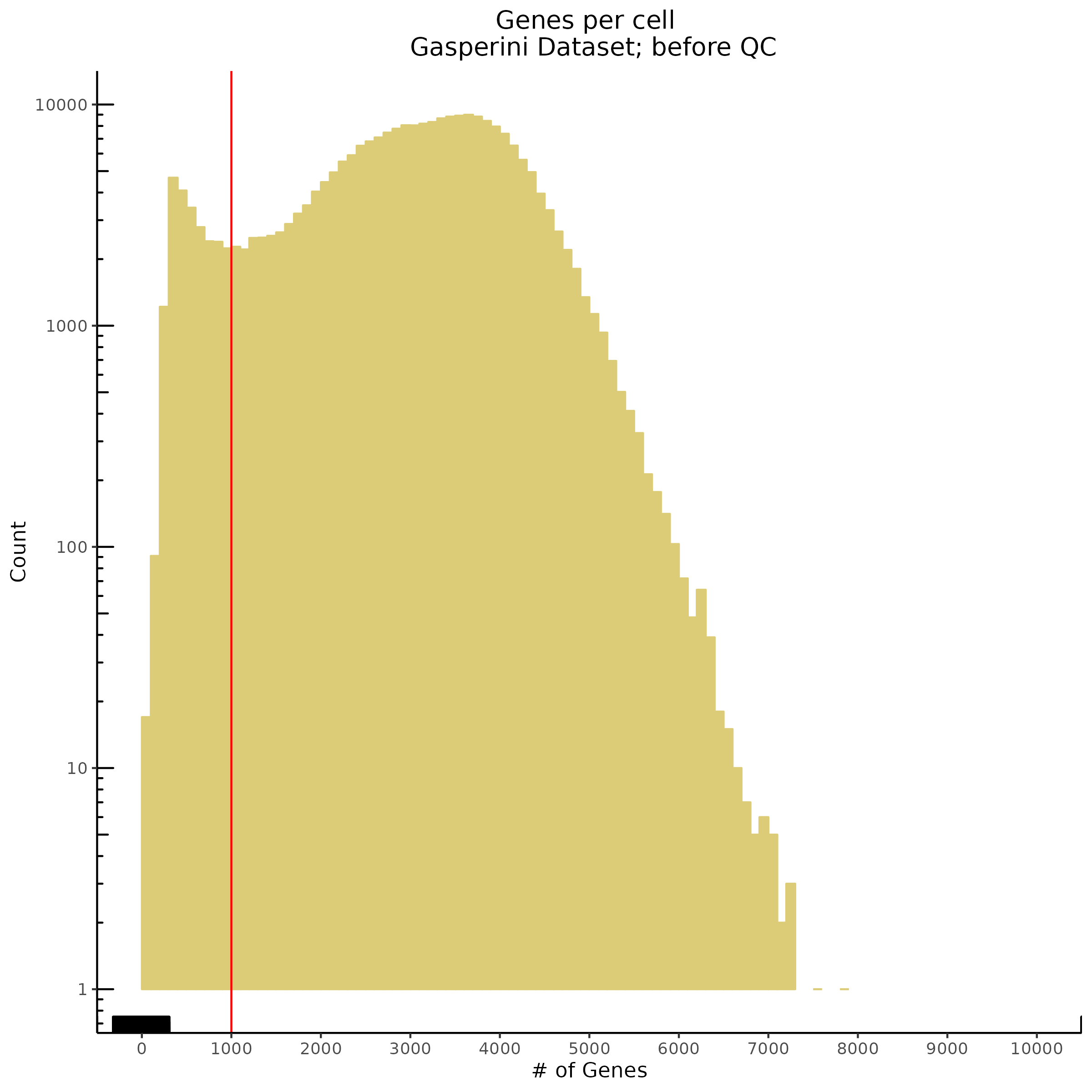
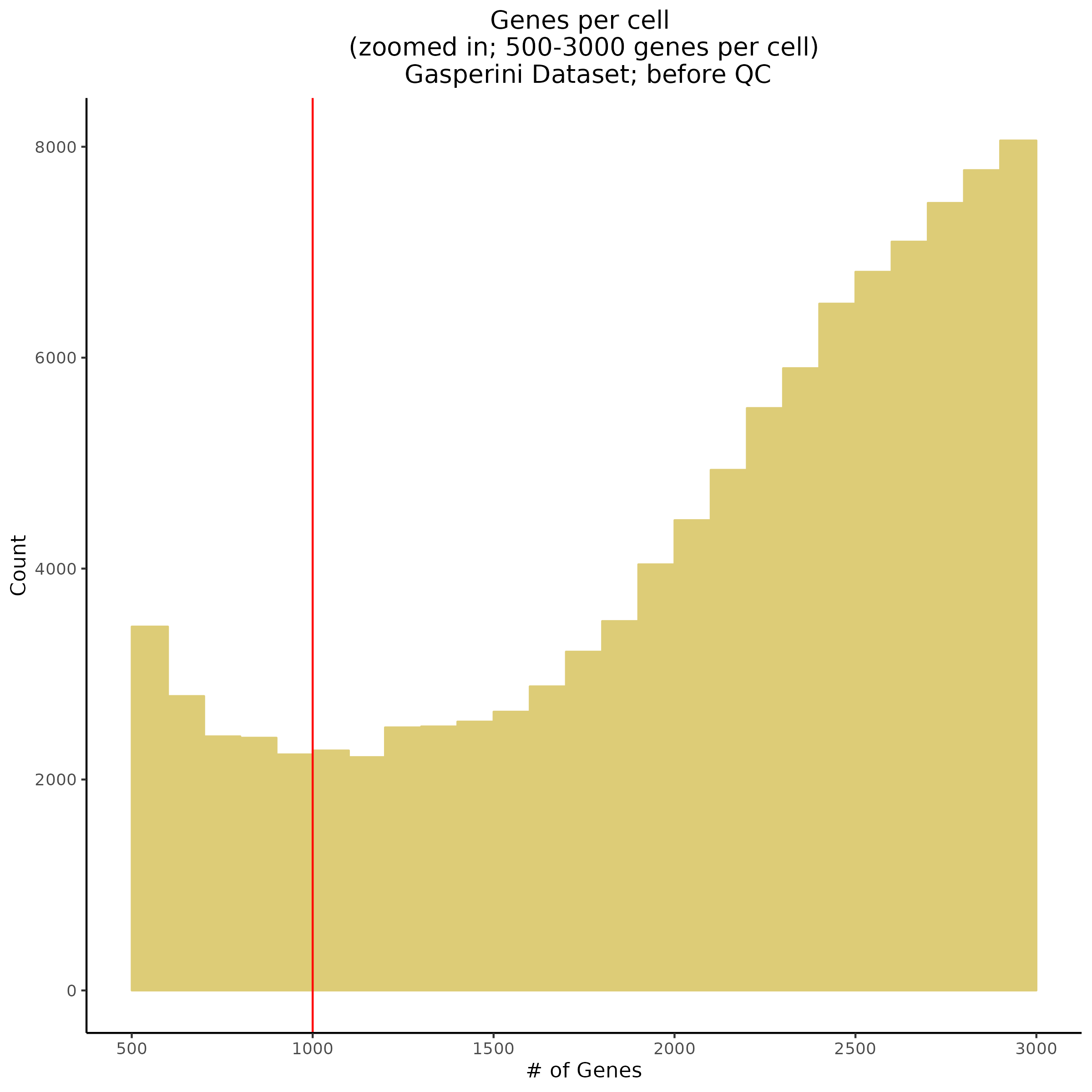
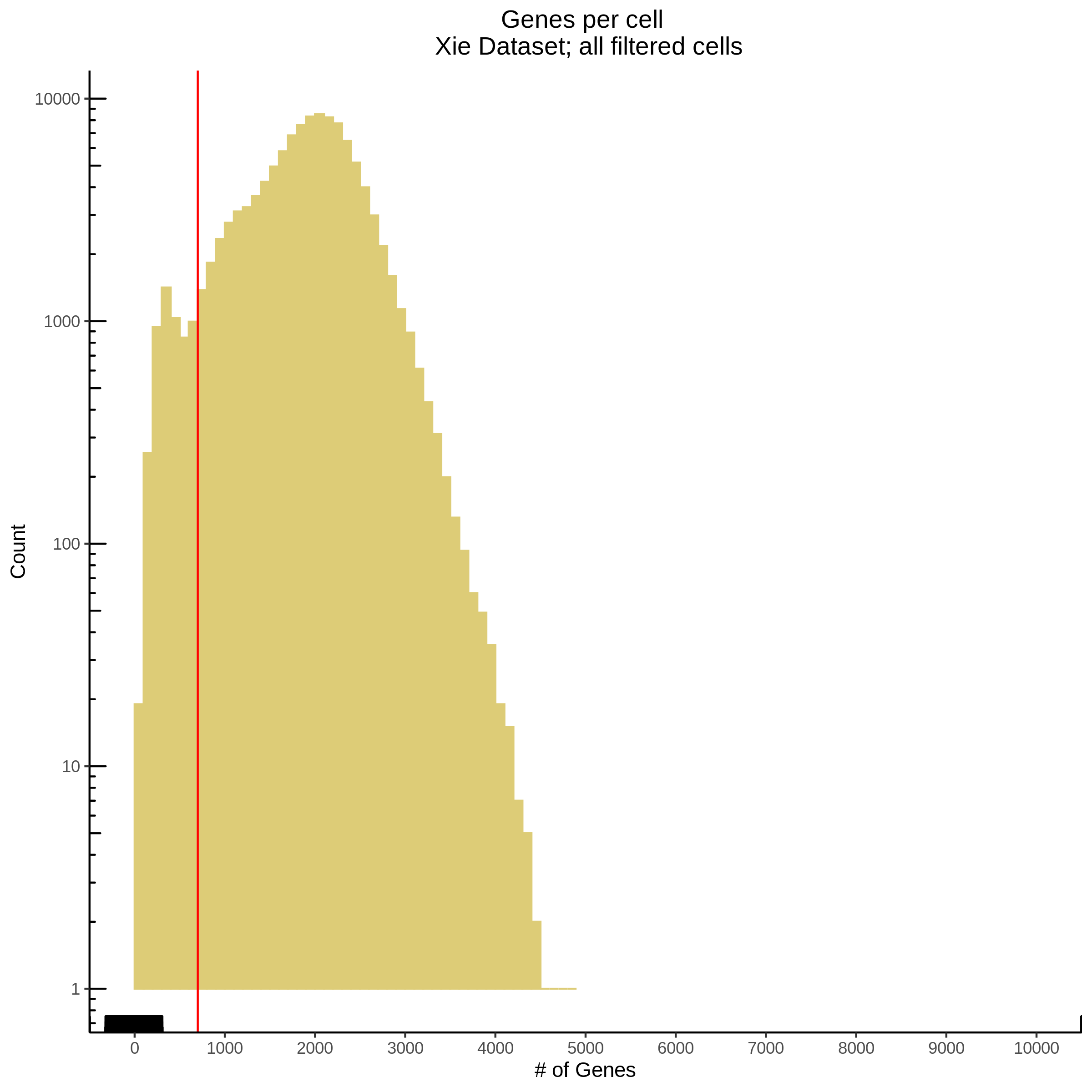
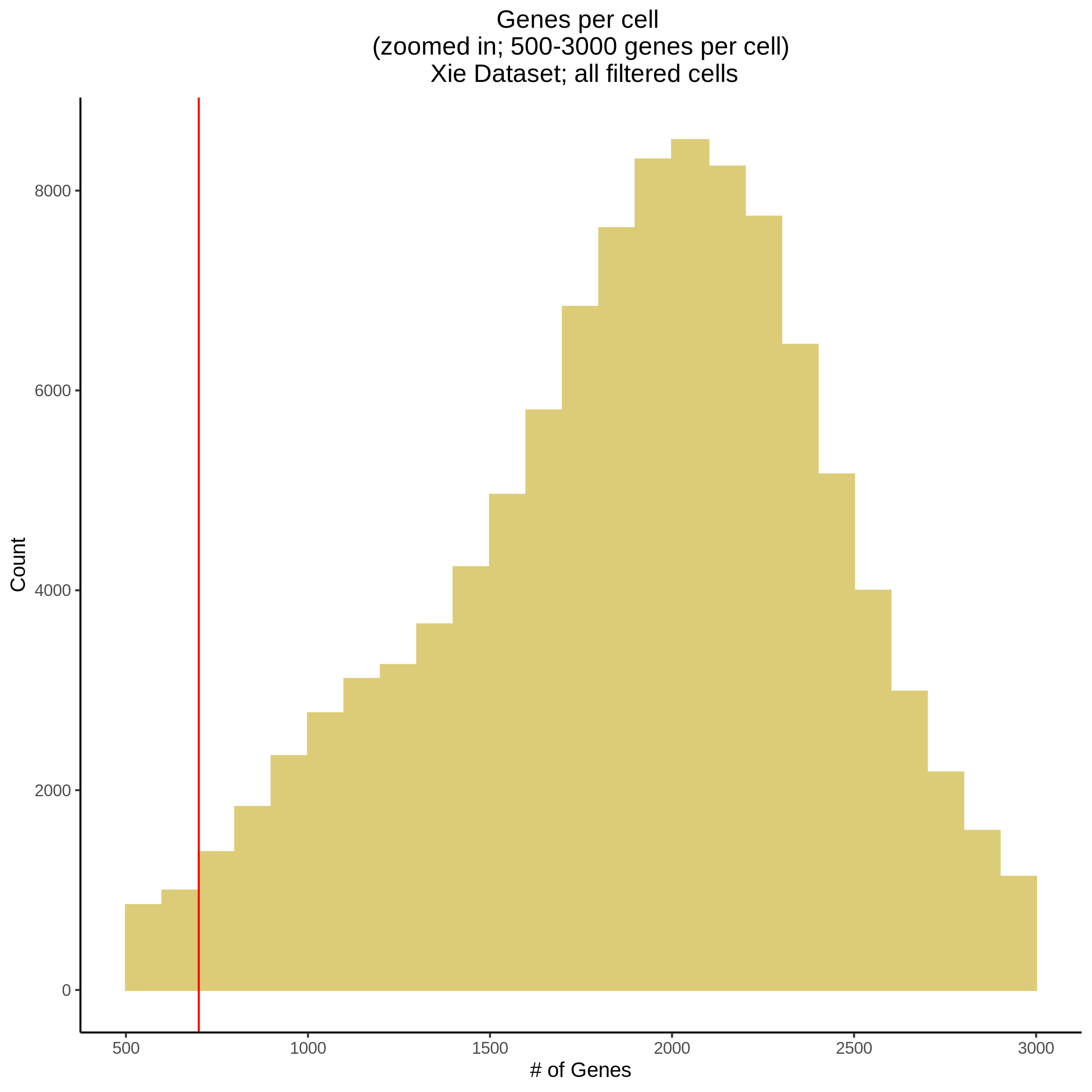
- Plot showing number # of genes per cell, another plot is made to focus on the 500-3000 critical region. A red line is placed at 700 genes per cell.
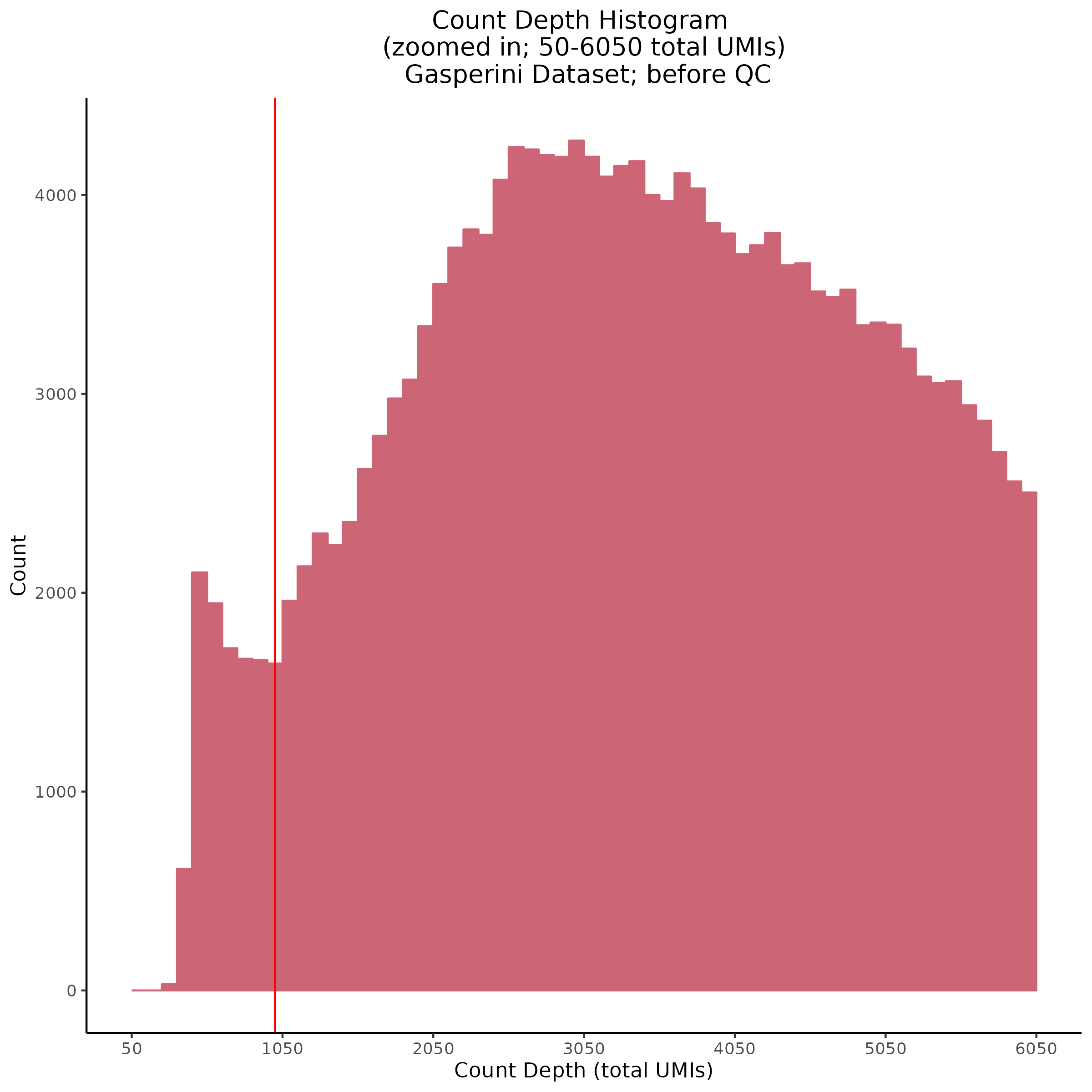
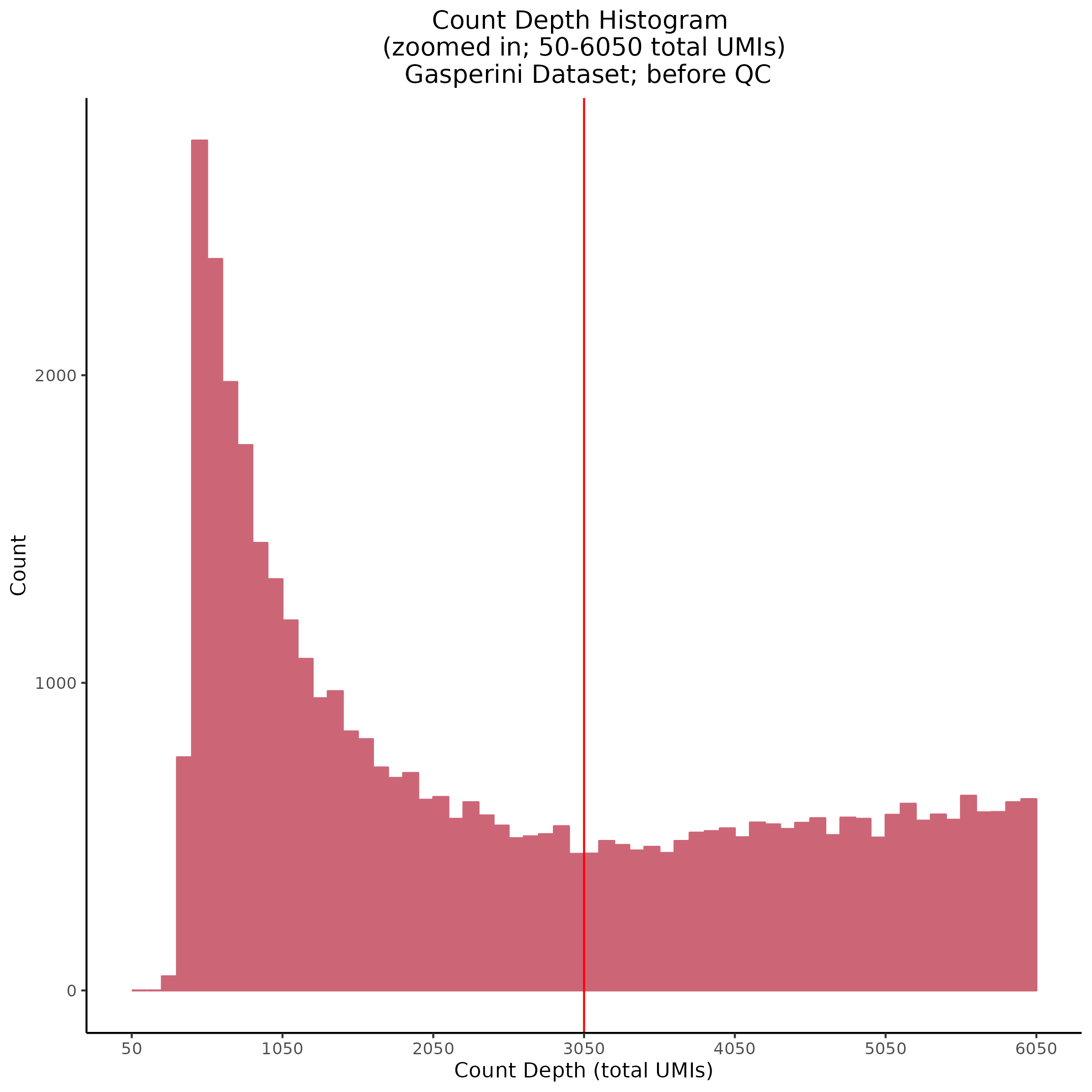
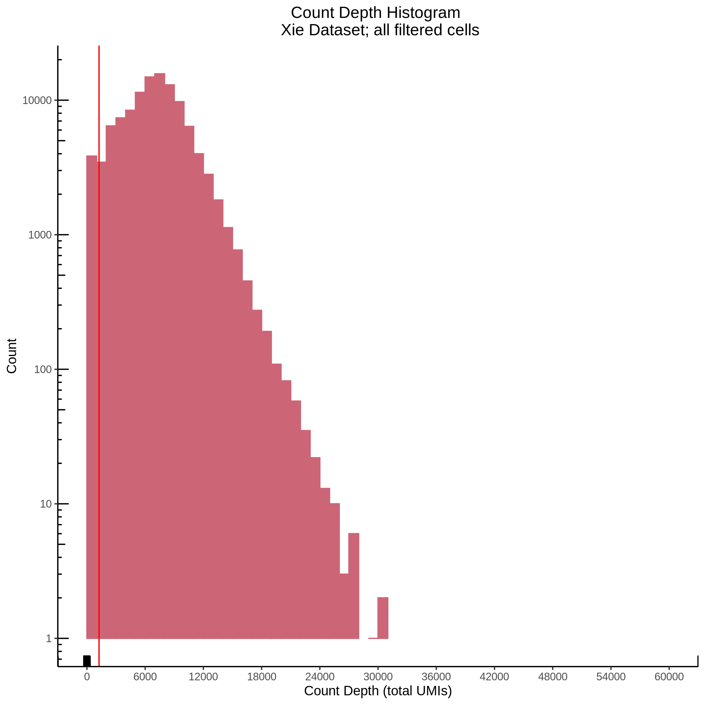
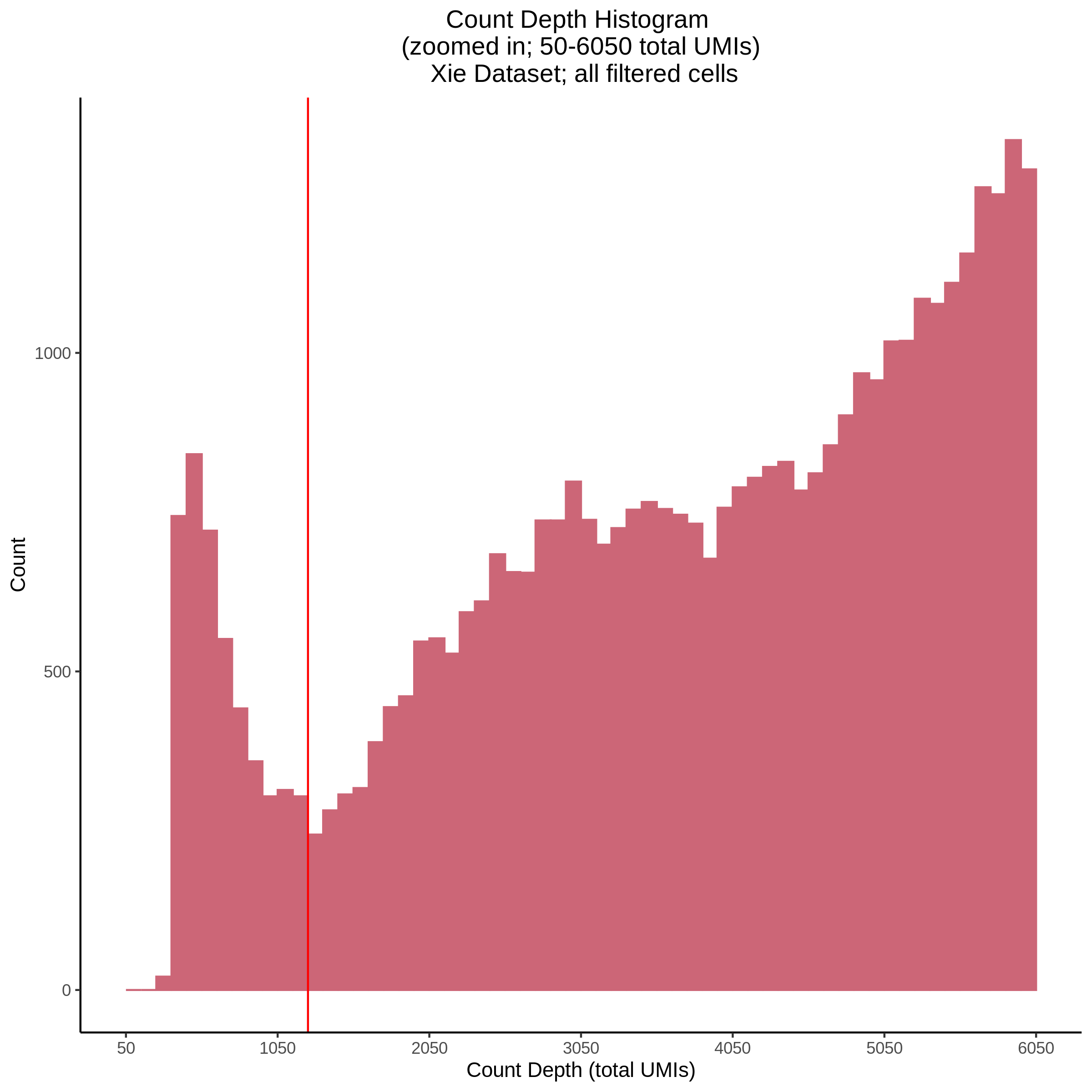
- Plot showing count depth (# of UMIs per cell) as a histogram. Another plot is made to focus on the 50-6050 total UMI count region. A red line is placed at 1100 UMIs.
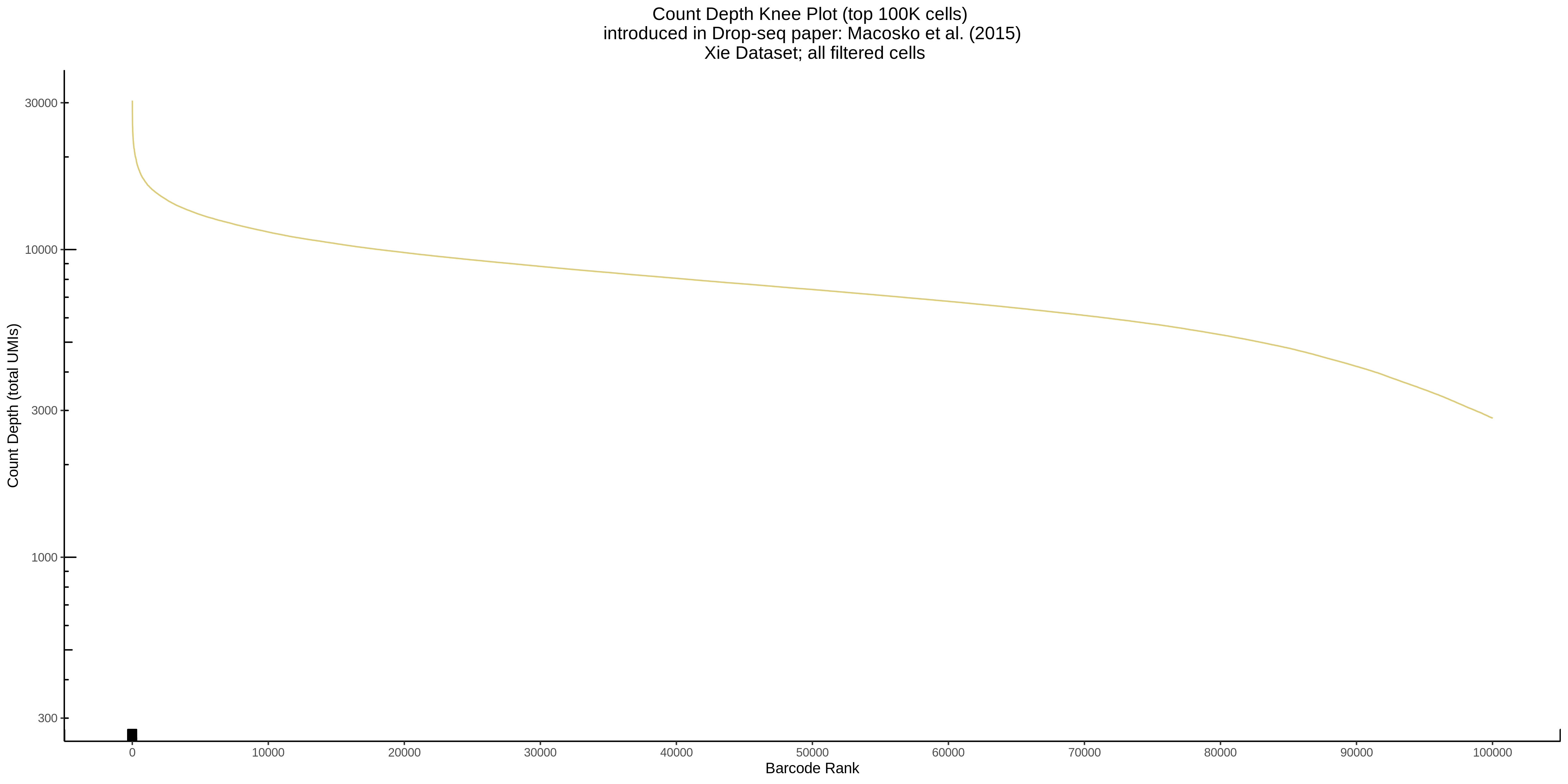
- Plot showing a count depth knee plot. This is a plot of the count depth vs ranked barcodes (based count depth per barcode). The plot itself was introduced originally in the Drop-seq paper (Macosko et al., Highly parallel genome-wide expression profiling of individual cells using nanoliter droplets, 2015.) Here you rank cells based on count depth to produce a count depth (total UMIs) vs barcode rank plot and place a horizontal threshold where the line curves down steeply. This plot shouldnt contain a sharp decreasing ‘knee’ or curve down steeply becuase cellranger has already performed this filtering. We are making this plot as a check on cellranger’s work.
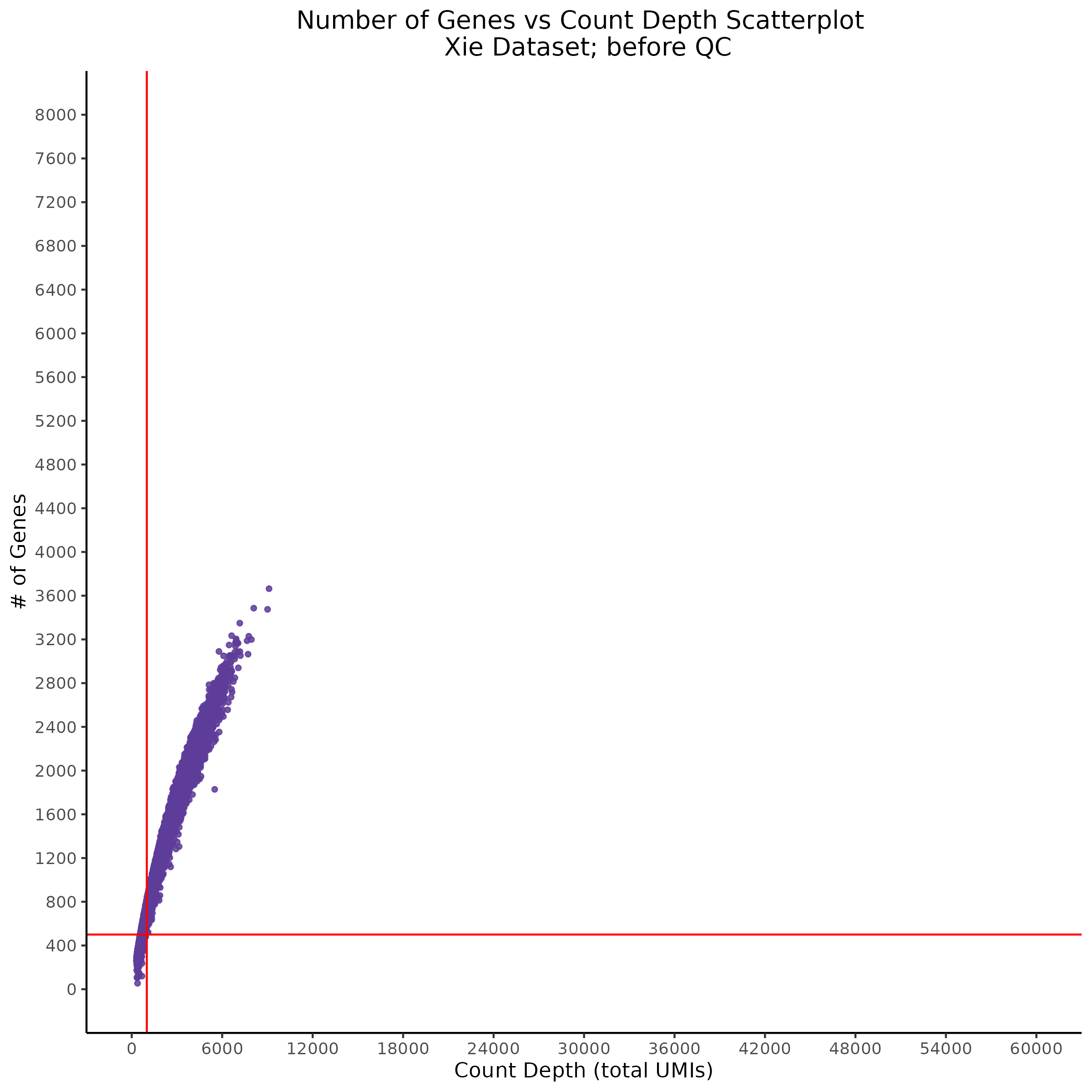
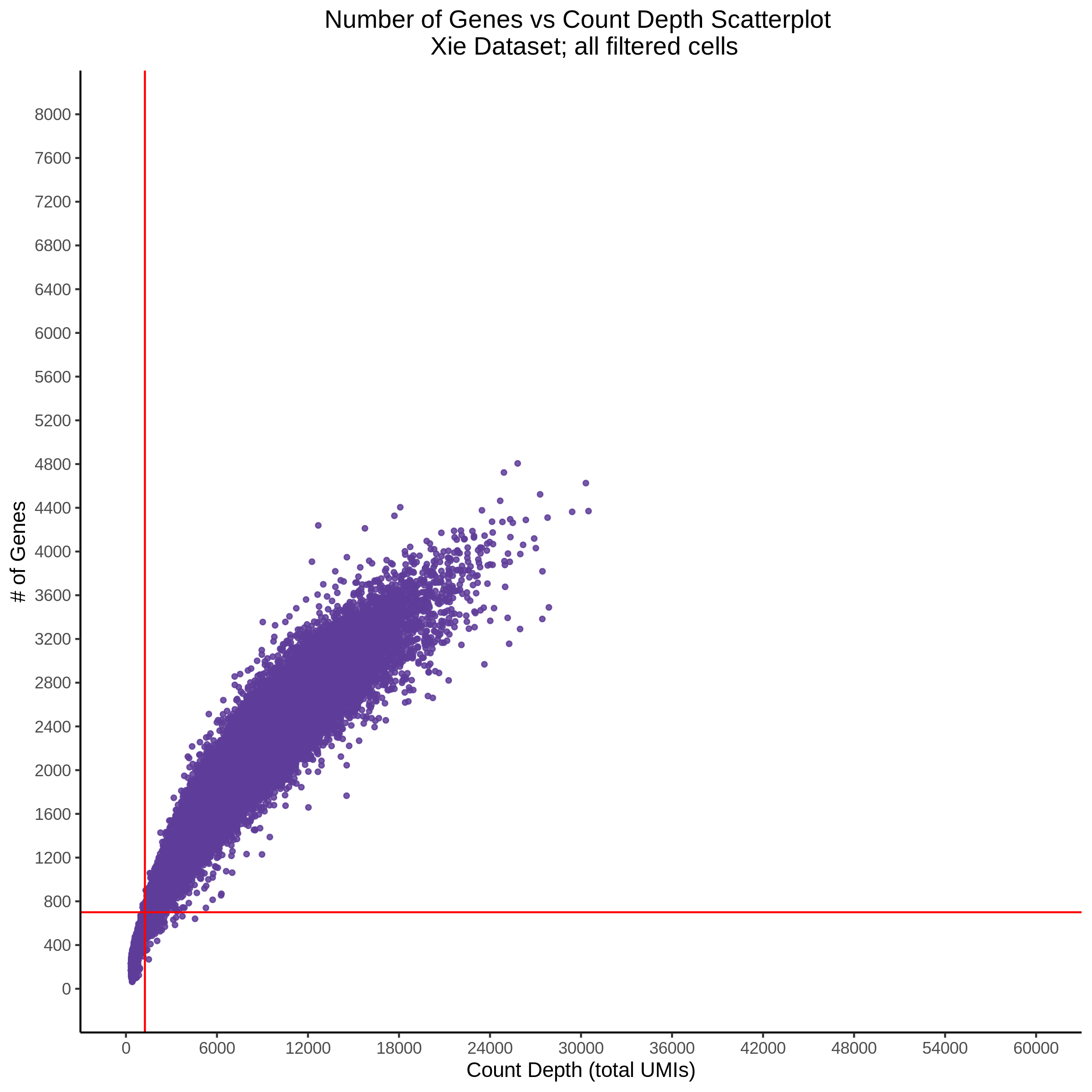
- Scatterplot showing count depth (total UMIs) vs # of genes. This combines plots 3 and 4 above. Red lines are placed on each of the appropriate QC thresholds.
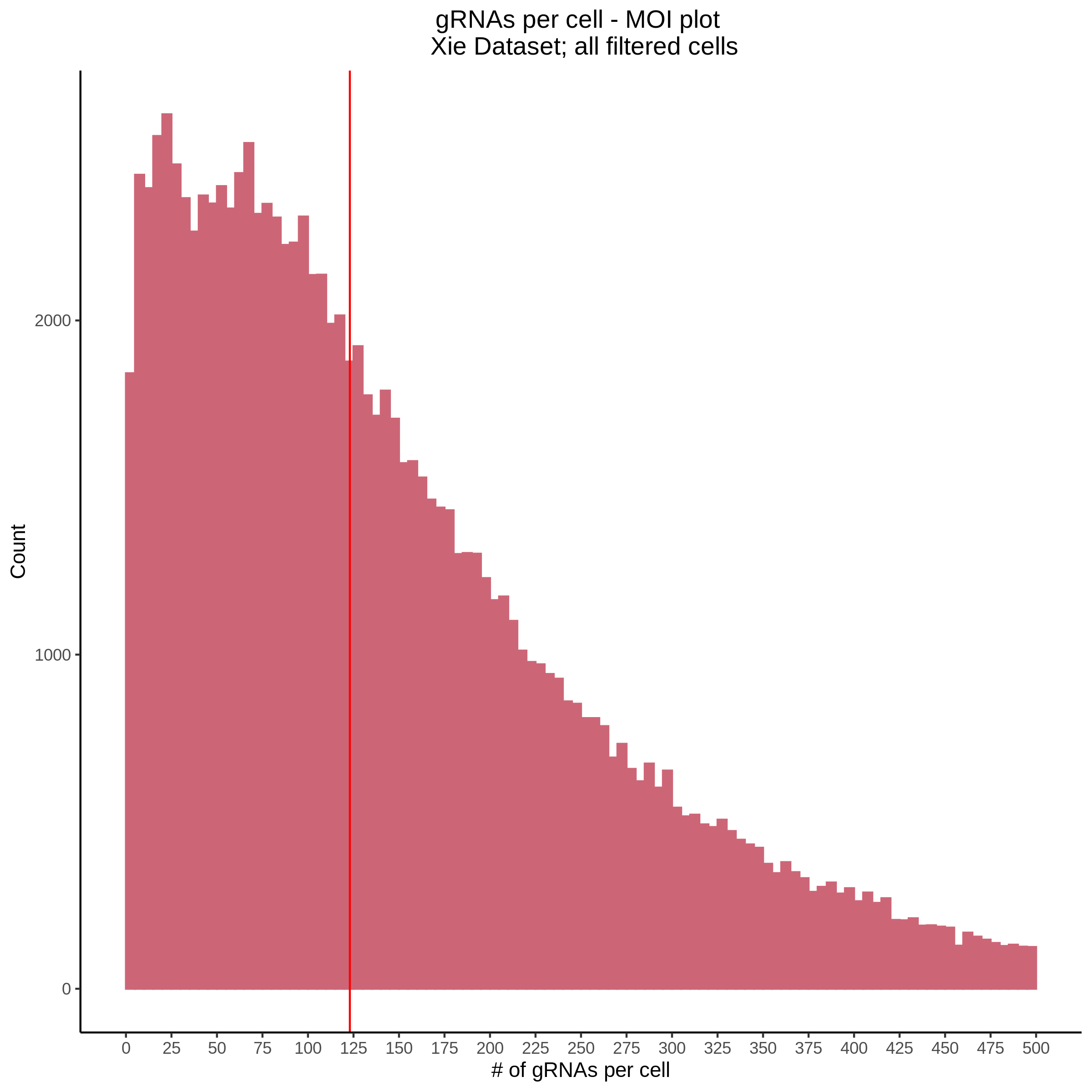
- Histogram showing sgRNAs per cell. This is meant to show the initial MOI and distribution within the pre-QC dataset. A red line is placed at the median or MOI estimate.
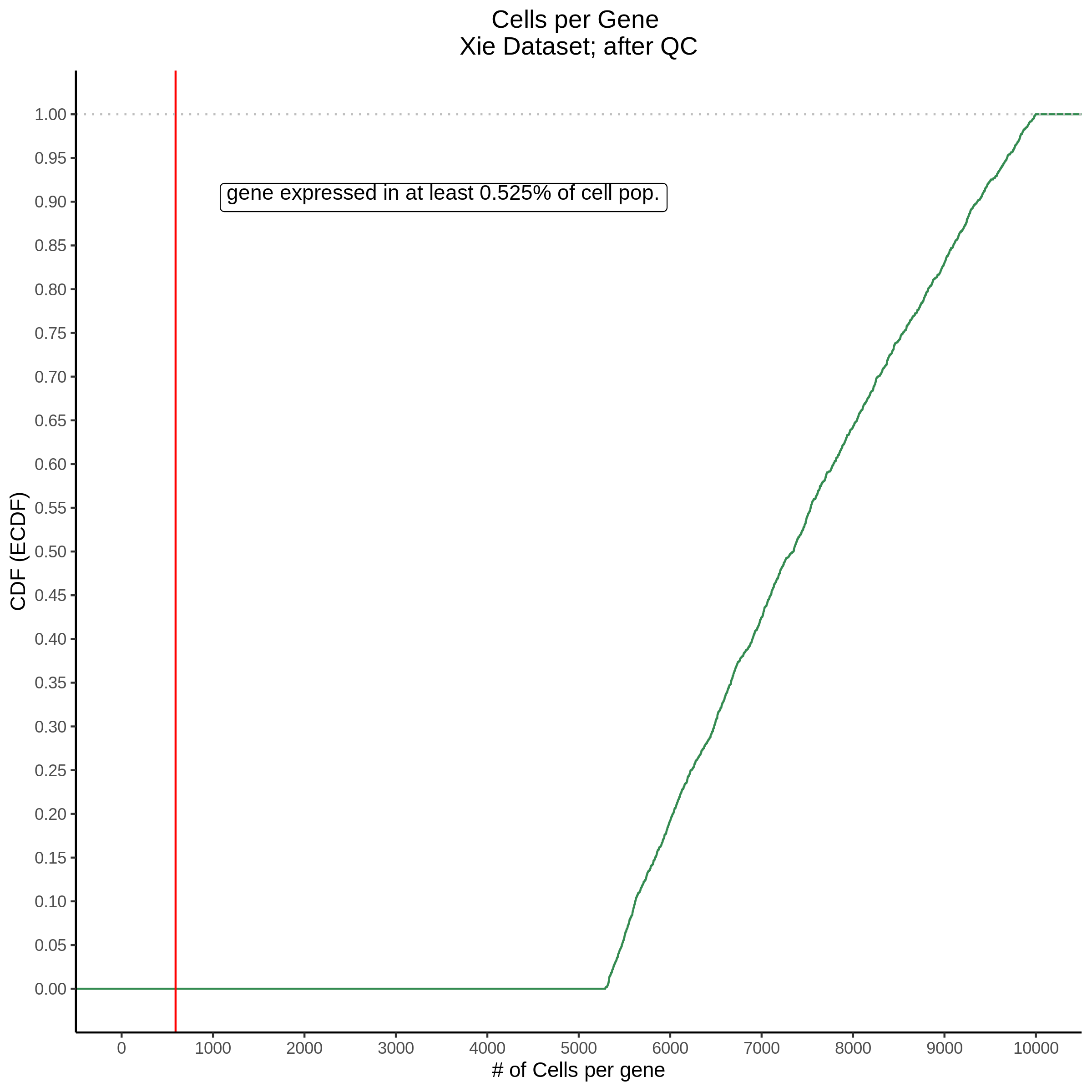
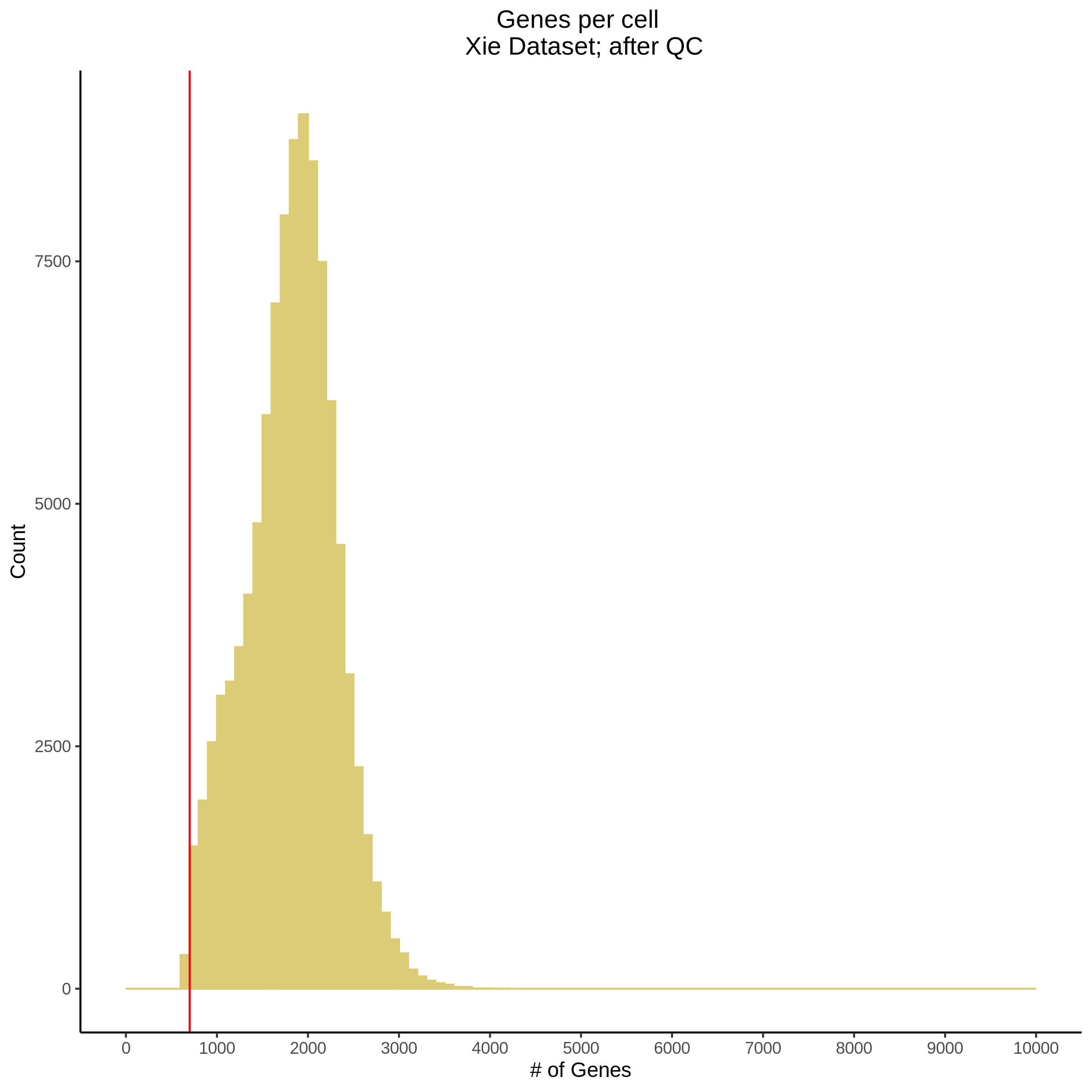
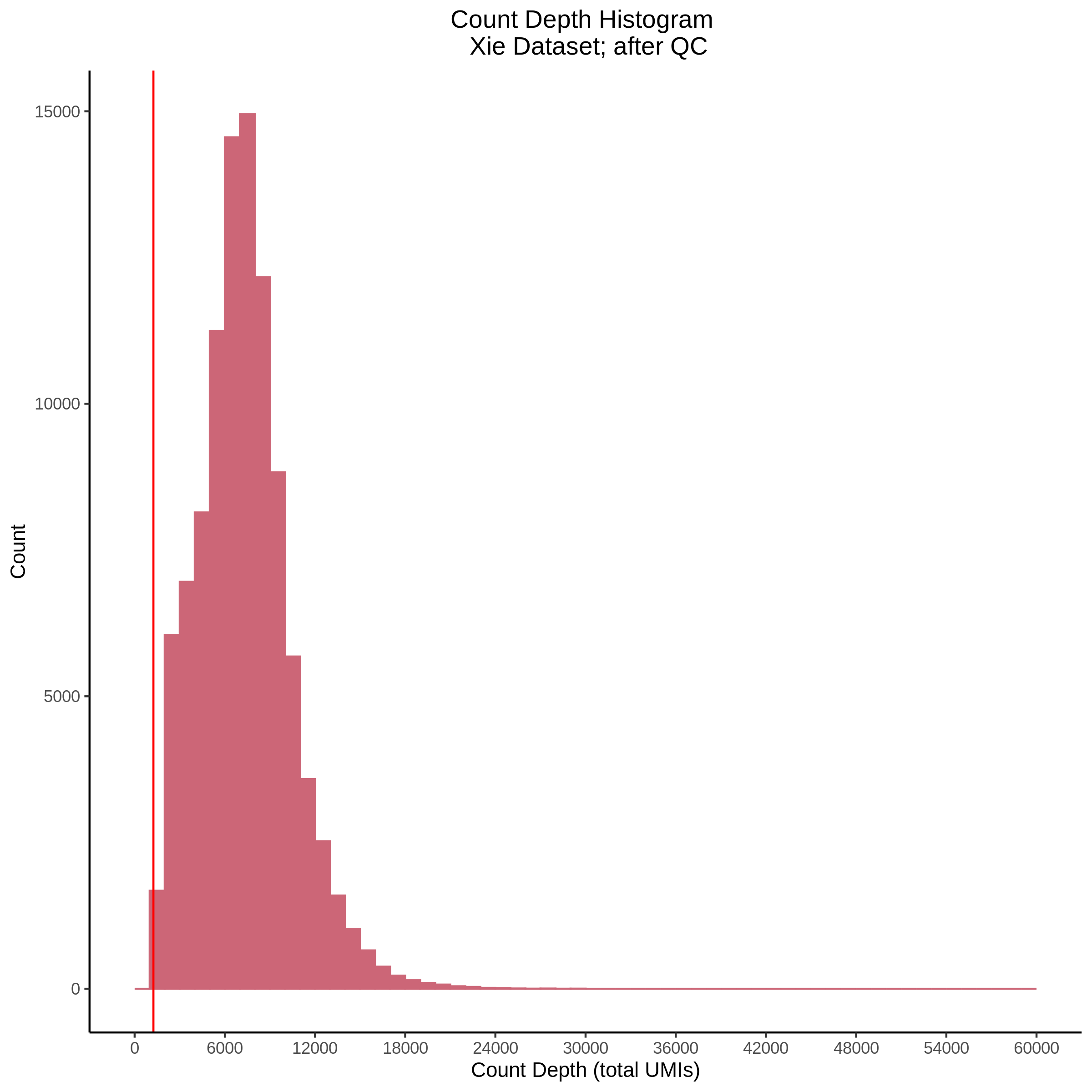
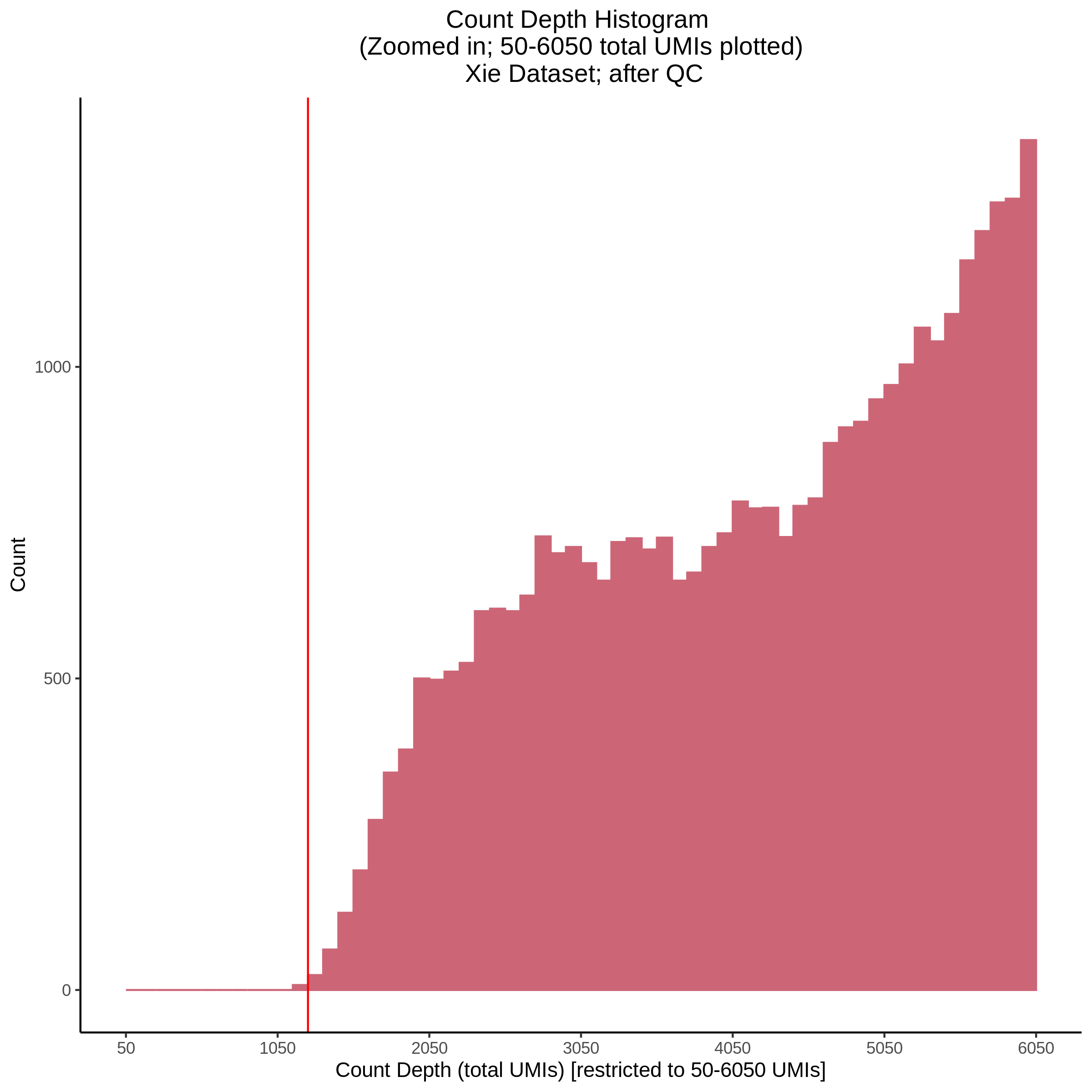
QC Plot-Results after QC:
These QC plots serve to highlight the same plots shown above applied to the final, filtered and prepared dataset.
- Plot showing the percent of mitochondrial reads in all cells before QC. A red line is placed at 20%, the threshold for mitochondrial contaminated cells.
- Plot showing cells per gene in CDF plot, a red line is placed at .0525% of total cells.
- Plot showing number # of genes per cell, another plot is made to focus on the 500-3000 critical region. A red line is placed at 700 genes per cell.
- Plot showing count depth (# of UMIs per cell) as a histogram. Another plot is made to focus on the 50-6050 total UMI count region. A red line is placed at 1100 UMIs.
- Plot showing a count depth knee plot. This is a plot of the count depth vs ranked barcodes (based count depth per barcode). The plot itself was introduced originally in the Drop-seq paper (Macosko et al., Highly parallel genome-wide expression profiling of individual cells using nanoliter droplets, 2015.) Here you rank cells based on count depth to produce a count depth (total UMIs) vs barcode rank plot and place a horizontal threshold where the line curves down steeply. This plot shouldnt contain a sharp decreasing ‘knee’ or curve down steeply becuase cellranger has already performed this filtering. We are making this plot as a check on cellranger’s work.
- Scatterplot showing count depth (total UMIs) vs # of genes. This combines plots 3 and 4 above. Red lines are placed on each of the appropriate QC thresholds.
- Histogram showing sgRNAs per cell. This is meant to show the initial MOI and distribution within the pre-QC dataset. A red line is placed at the median or MOI estimate.
gene-gRNA pairs for SCEPTRE
In order to run SCEPTRE we also need to generate gene-grna pairs based on both the filtered genes and gRNAs above. This is done in a seperate script because it takes a lot of memory. One other thing that is important to note, is that we need information about the sgRNAs in order to calculate trans- distances. Notice that we build on the CSV reference made during the cellranger prep.
gRNA_location_ref = data.table::fread('/home/nbabushkin/xie_mappability_sceptre/xie_feature_reference_m1_INFO.csv', stringsAsFactors = F, header = T, sep=',')
# header: id,name,read,pattern,sequence,feature_type,region_pos_hg38,spacer_pos_hg38
# chr1:11671358-11671758, chr1:11671483-11671502

# extract chromosome info
gRNA_location_ref = gRNA_location_ref %>% rowwise() %>% dplyr::mutate(chr = str_replace( strsplit(spacer_pos_hg38, ":")[[1]][1], 'chr', '' ))

# extract start and stop
gRNA_location_ref = gRNA_location_ref %>% rowwise() %>% dplyr::mutate(start = strsplit( strsplit(spacer_pos_hg38, ":")[[1]][2], '-' )[[1]][1] )
gRNA_location_ref = gRNA_location_ref %>% rowwise() %>% dplyr::mutate(end = strsplit( strsplit(spacer_pos_hg38, ":")[[1]][2], '-' )[[1]][2] )

# fix names used in matrices vs those used in the reference
gRNA_location_ref = gRNA_location_ref %>% rowwise() %>% dplyr::mutate(id = str_replace_all(id, '_', '-'))

# clean up the frame: rm non-autosomal gRNAs
temp = nrow(gRNA_location_ref)
gRNA_location_ref = gRNA_location_ref %>% dplyr::filter( chr %in% approved_chrs) # should be only 1-22
print(paste0('Removed ', (temp - nrow(gRNA_location_ref)), ' gRNAs from gRNA reference due to non-autosomal chr location'))

# clean up the frame NAs; expected result: 0 removed
temp = nrow(gRNA_location_ref)
gRNA_location_ref = gRNA_location_ref %>% na.omit() # cannot be NA
print(paste0('Removed ', (temp - nrow(gRNA_location_ref)), ' gRNAs from gRNA reference due NA values'))

# clean up filtered out gRNAs
temp = nrow(gRNA_location_ref)
gRNA_location_ref = gRNA_location_ref %>% dplyr::filter( id %in% ondisc_gRNAs) # should be only 1-22
print(paste0('Removed ', (temp - nrow(gRNA_location_ref)), ' gRNAs from gRNA reference due filtered out gRNAs'))

data.table::fwrite(gRNA_location_ref, file = paste0(out_dir, '/gRNA_location_reference.csv'), quote=F,row.names=F, sep=',') ##### |||||  write
Afterwards we can construct the pairs by calculating distances between the sgRNAs and a given gene. In order to do this efficiently, I load the reference into the a GRanges object, then perform an overlap search for each given sgRNA. Overlaps are then inverted to identify genes outside of 10 Mb.
Totals / Summary
- The final size of the cDNA matrix: An integer-valued ondisc_matrix with 7112 features and 100682 cells.
- The final size of gRNA matrix: An integer-valued ondisc_matrix with 5142 features and 100682 cells.
- A total of 34,989,109 trans- gene-gRNA pairs for SCEPTRE analysis.
Xie et al. Dataset Alignment+Counting using CellRanger
With the arrival of a new cellranger version recently it became posssible to perform both single cell transcriptome sequencing alignment/counting alongside CRISPR feature barcode extraction. As a result, it is not longer necessary to strictly use tools such as UMI-tools to count and extract CRISPR feature barcode data from the sgRNA amplified raw data.
This section will go over the neccessities for setting up and generating cDNA/GDO matrices for the Xie et al dataset, starting from the raw data on GEO all the way through to final, filtered and aggregated cDNA/GDO matrices that are ready for further analysis such as QC and preperation for SCEPTRE.
Before this section begins, theres another section below on 7/7/2022 that discussed the batches and cellranger reagents used in generating the raw sequencing data.
In order to set up CellRanger we need to understand two main aspects about the dataset:
- How are the batches set up?
- What are the sgRNA sequences and position in read?
For 1), we know that Xie et al. is structured to use 5 batches which were sequenced using 10 runs (1_1, 1_2, 2_1…5_2) and based on CellRanger documents we know that each sequencing run should be counted seperately: “first step is to run cellranger count…on each individual GEM well prepared”. Then each run is combined using the aggregation function. This is found on the cellranger documentation here: https://support.10xgenomics.com/single-cell-gene-expression/software/pipelines/latest/using/aggregate
This means that we need to set up library CSV files specific to each GEM well as we need CSV inputs for each of the cellranger count commmands we make. An example for batch1_1 is shown below:
fastqs,sample,library_type
.../data/Xie_raw_data/,cDNA1_1,Gene Expression
.../data/Xie_raw_data/,GDO1_1,CRISPR Guide Capture
For 2) you must get to know a bit about the cellranger CRISPR feature barcode extraction and the data you are working with. Firstly, cellranger feature barcode extraction requeres not only the sgRNA protospacer sequence but also its position in READ 2 of the sgRNA amplified GDO raw data. What this means is that we need to understand were exactly within R2 of the sequencing data the barcode is being captured since Xie et al. is using MOSIAC-Seq, an inhouse CRISPR barcoding solution. It is important to realize that although it may appear that Xie et al. is using 10xv2 reagents in order to generate the sequencing data, that only applies to the cDNA data - and not at all to the CRISPR feature barcode data. It would thus be incorrrect to use the CRISPR feature baracode patterns suggested on the Cellranger website for 10xv2 reagents. That pattern is only relevant to datasets where the feature barcode data also uses 10xv2 technology.
In order to determine this using only the data provided I reccomend performing a FBA QC analysis using the FBA tool.
FBA Analysis of Xie et al. Raw Data
In order to setup FBA we need to first gather a set of barcodes and a sgRNA sequences table. The barcodes we can be taken from filtered data sepecific to the batch. I choose to run on batch 1_1 so I used filtered barcodes from GEO. For the sgRNA input for FBA we need a TSV file, no header, detailing id and protospacer sequence.
Here is the first few lines of my FBA sgRNA input:
GHSGRNALIB_1702_00001   TTCAGTTTGCCTTACTCGT
GHSGRNALIB_1702_00002   TGAACCTACCAGGCTTGCG
GHSGRNALIB_1702_00003   CTTGCGTGGAGGGGACAGA
GHSGRNALIB_1702_00004   GTCCTCTCTGCGAAGCTCG
GHSGRNALIB_1702_00005   TCCTCTCTGCGAAGCTCGA
GHSGRNALIB_1702_00006   TCCCTCGAGCTTCGCAGAG
GHSGRNALIB_1702_00007   GGGATCACTGAAGCAGGCC
GHSGRNALIB_1702_00008   GGGCAGTTAAGATAAGCCA
GHSGRNALIB_1702_00009   AGGCATCTGTCCGTAAGCT
And the barcodes (borrowed from filtered data, make sure to trim OFF the batch number since FBA expects no cellranger batch id (example: AAACCTGAGGAGTACC-1)):
AAACCTGAGAGCTTCT
AAACCTGAGATCCCAT
AAACCTGAGCGTCTAT
AAACCTGAGCTAGTCT
AAACCTGAGGACACCA
AAACCTGAGGAGTACC
AAACCTGAGGAGTTTA
AAACCTGAGGCCATAG
AAACCTGAGTATCGAA
Then we can run FBA like so:
    fba qc -t 12 -n 333000 \
        -1 /project/xuanyao/nikita/SCEPTRE/data/Xie_raw_data/GDO1_S1_L001_R1_001.fastq.gz \
        -2 /project/xuanyao/nikita/SCEPTRE/data/Xie_raw_data/GDO1_S1_L001_R2_001.fastq.gz \
        -w /home/nbabushkin/xie_mappability_sceptre/count1_filtered_barcodes_clean.tsv \
        -f /home/nbabushkin/xie_mappability_sceptre/xie_feature_sgRNAs_FBA_input.tsv \
        --output_directory /home/nbabushkin/xie_mappability_sceptre/Xie_GDO_fbaQC_large \
        -cb_m 1 \
        -fb_m 1
Here you can see that we provide the raw data in the form of gziped FASTQ files, the baracodes, the sgRNAs sequences, set a hamming distance of 1, and sample only 333,000 random R1/R2 reads in order to make this a bit faster.
From the results we want to focus our attention to the base content of R2 since that is the read that will contain our sgRNA protospacer sequence within the sgRNA amplified data.
TEST
Inspecting this further should show that the our barcodes are likely located between position 19 and position 38 in read 2. In order to generate the sgRNA reference for CellRanger we can thus do the following:
# CELLRANGER REFERENCE
excel_XIE_sgRNA_data = pandas.read_excel('/project/xuanyao/nikita/SCEPTRE/data/Xie_2019/TABLES1.xlsx', sheet_name=0)
ids = excel_XIE_sgRNA_data['ID'].tolist()
cids = [idd.replace(':', '_') for idd in ids]
seqs = excel_XIE_sgRNA_data['spacer sequence'].tolist()
pattern = '5P'+'N'*19+'(BC)'
patterns = [pattern]*len(ids)
reads = ['R2'] * len(ids)
ftypes = ['CRISPR Guide Capture']* len(ids)
cellranger_cols = ['id',    'name', 'read', 'pattern',  'sequence', 'feature_type']
df = pandas.DataFrame(list(zip(cids, cids, reads, patterns, seqs, ftypes)), columns=cellranger_cols)
ref_cols = ['id',   'name', 'read', 'pattern',  'sequence', 'feature_type', 'region_pos_hg38','spacer_pos_hg38']
df_ref = pandas.DataFrame(list(zip(cids, cids, reads, patterns, seqs, ftypes, excel_XIE_sgRNA_data['region pos (hg38)'].tolist(), excel_XIE_sgRNA_data['spacer pos (hg38)'].tolist())), columns=ref_cols)
ss = df.size
temp = df.drop_duplicates(subset=['sequence'], keep=False) # drop both duplicates, keep neither sgRNA
if temp.size < ss:
    print('duplicates removed: {}'.format(ss - temp.size))
dups = df[df.duplicated(['sequence'], keep=False)]['sequence'].tolist()
df[df.duplicated(['sequence'], keep=False)]
ref = df.drop_duplicates(subset=['sequence'], keep='first')
ref_ref = df_ref.drop_duplicates(subset=['sequence'], keep='first')
ref.to_csv('/home/nbabushkin/xie_mappability_sceptre/xie_feature_reference_m19.csv', sep=',', header=True, index=False)
ref_ref.to_csv('/home/nbabushkin/xie_mappability_sceptre/xie_feature_reference_m19_INFO.csv', sep=',', header=True, index=False)
This code does several things:
- It creates the CellRanger sgRNA feature reference called: xie_feature_reference_m19.csv. This is specifically formated.
- It creates a larger more detailed copy of the reference called: xie_feature_reference_m19_INFO.csv which retains helpful information.
- It identifies and filters duplicated protospacer sequences becuase cellranger requires 1:1 uniqueness between sgRNA id and protospacer sequence. We thus take the first of 720 duplicated sequences.
- It tables the duplicated sequences for backup in a dataframe: dups.
- It creates a sgRNA extraction pattern compatable with Cellranger: pattern = ‘5P’+‘N’*19+‘(BC)’
Something really important is the pattern:
pattern = '5P'+'N'*19+'(BC)' This can be tricky becuase we need to remember that cellranger is written and implemented in Python! Why is this important?
Well, Python is 0 based while R is 1 based. What this means is that positional data in python is offset due to 0 being the first index position. For example, the Nth element of a list is accessed by list[N-1]. In R, the Nth element is simply list[N]. This difference means that if you are using a custom feature barcode experiment, such as MOSIAC-Seq used by Xie et al., and not 10xv2/10xv2 reagents for feature barcodes you must take this into account since Cellranger will interpret and create a REGEX expression within python based on pythonic definition of positions.
As a result, if our sgRNA protospacers must match with a hamming distance of 1 to positions (19:38) in READ 2, the 19th position would have 19 nucleotides before it placing those nucleotides pythonically at positions 0 through 18 (19 total nucleotides). Then the 19th position starts the actual barcode.
pattern = '5P'+'N'*19+'(BC)'
Another way of looking at this is to realize that we need to pad the pattern by 1 nucleotides to offset the fact that 19:38 is actually zero based both in FBA and in Cellranger (but not in R).
Putting it all together: Running CellRanger Count
Now that we have addressed both 1) and 2) from above, we are ready to run cellranger count:
Cellranger Count cmd example:
/home/nbabushkin/cellranger-7.0.1/cellranger count  --disable-ui --include-introns false --no-bam --nosecondary --localcores=48 --localmem=128 --id=gemgroup1_1 \
         --transcriptome=/project/xuanyao/nikita/SCEPTRE/cellranger_refs/GRCh38-2020-A_build/cellranger_GRCh38reference \
         --libraries=/home/nbabushkin/xie_mappability_sceptre/gemgroup_libraries/1_1libraries.csv --feature-ref=/home/nbabushkin/xie_mappability_sceptre/xie_feature_reference_m19.csv
Aggregating Cellranger Counts:
One thing to note is that while this is very straightforward and easy, cellranger aggregate has two downsides at the moment:
- Aggregation for CRISPR barcodes calls a protospacer step within cellranger which can take betwen 8-12 hours.
- Aggregation uses a lot of memory and I found it necessary to all the memory on a node (~160 GB)
Aggregation CSV (aggr_paths_m19_batched.csv):
sample_id,molecule_h5
gemgroup1_1,/scratch/midway3/nbabushkin/Xie_gemgroup_count_m19/gemgroup1_1/outs/molecule_info.h5
gemgroup1_2,/scratch/midway3/nbabushkin/Xie_gemgroup_count_m19/gemgroup1_2/outs/molecule_info.h5
gemgroup2_1,/scratch/midway3/nbabushkin/Xie_gemgroup_count_m19/gemgroup2_1/outs/molecule_info.h5
gemgroup2_2,/scratch/midway3/nbabushkin/Xie_gemgroup_count_m19/gemgroup2_2/outs/molecule_info.h5
gemgroup3_1,/scratch/midway3/nbabushkin/Xie_gemgroup_count_m19/gemgroup3_1/outs/molecule_info.h5
gemgroup3_2,/scratch/midway3/nbabushkin/Xie_gemgroup_count_m19/gemgroup3_2/outs/molecule_info.h5
gemgroup4_1,/scratch/midway3/nbabushkin/Xie_gemgroup_count_m19/gemgroup4_1/outs/molecule_info.h5
gemgroup4_2,/scratch/midway3/nbabushkin/Xie_gemgroup_count_m19/gemgroup4_2/outs/molecule_info.h5
gemgroup5_1,/scratch/midway3/nbabushkin/Xie_gemgroup_count_m19/gemgroup5_1/outs/molecule_info.h5
gemgroup5_2,/scratch/midway3/nbabushkin/Xie_gemgroup_count_m19/gemgroup5_2/outs/molecule_info.h5
CellRanger Aggregate cmd example:
time /home/nbabushkin/cellranger-7.0.1/cellranger aggr --nosecondary --disable-ui --id=AGG_MOSIAC_SEQ --localcores=48 --localmem=160 \
    --csv=/home/nbabushkin/xie_mappability_sceptre/aggr_paths_m19_batched.csv
Configuring CellRanger for Midway3
In this section I will go over how to configure cellranger to submit jobs to the Midway3/Midway2 clusters (make your system Admin happy).
Briefly, as an introduction it is worth mentioning that this arose out to neccessity becuase of the sheer compute power necessary to process the KD8 dataset published by Replogle. Specifically, I was able to generate counts for each gemgroup by spreading my CellRanger counts accross the sever with ample space for the temporary file usage (lots of small files, check your file capacity).
Here is the issue that I ran into specifically after about 12hrs into the aggregation function:
2022-10-04 18:59:40 [runtime] (update)          ID.AGGKD8.SC_RNA_AGGREGATOR_CS.COUNT_AGGR.SC_RNA_AGGREGATOR.NORMALIZE_DEPTH.fork0 chunks running (71/129 completed)
2022-10-04 19:05:53 [runtime] (update)          ID.AGGKD8.SC_RNA_AGGREGATOR_CS.COUNT_AGGR.SC_RNA_AGGREGATOR.NORMALIZE_DEPTH.fork0 chunks running (72/129 completed)
2022-10-04 19:11:53 [runtime] (update)          ID.AGGKD8.SC_RNA_AGGREGATOR_CS.COUNT_AGGR.SC_RNA_AGGREGATOR.NORMALIZE_DEPTH.fork0 chunks running (72/129 completed)
2022-10-04 19:17:54 [runtime] (update)          ID.AGGKD8.SC_RNA_AGGREGATOR_CS.COUNT_AGGR.SC_RNA_AGGREGATOR.NORMALIZE_DEPTH.fork0 chunks running (72/129 completed)
2022-10-04 19:24:20 [runtime] (update)          ID.AGGKD8.SC_RNA_AGGREGATOR_CS.COUNT_AGGR.SC_RNA_AGGREGATOR.NORMALIZE_DEPTH.fork0 chunks running (73/129 completed)
2022-10-04 19:30:18 [runtime] (update)          ID.AGGKD8.SC_RNA_AGGREGATOR_CS.COUNT_AGGR.SC_RNA_AGGREGATOR.NORMALIZE_DEPTH.fork0 chunks running (73/129 completed)
2022-10-04 19:36:18 [runtime] (update)          ID.AGGKD8.SC_RNA_AGGREGATOR_CS.COUNT_AGGR.SC_RNA_AGGREGATOR.NORMALIZE_DEPTH.fork0 chunks running (73/129 completed)
From these CellRanger Aggregate logs we see that we are getting “stuck” at the NORMALIZE_DEPTH stage - which in theory may be expected. From this we see that it takes a lot of time and there are over 129 steps.
We can configure cellranger to use a template creating a SLURM template like so:
#!/bin/bash
#SBATCH --job-name=__MRO_JOB_NAME__
#SBATCH --account=pi-\xuanyao
#SBATCH --partition=caslake
#SBATCH -N 1
#SBATCH -c __MRO_THREADS__
#SBATCH --mem=__MRO_MEM_GB__G
#SBATCH -o __MRO_STDOUT__
#SBATCH -e __MRO_STDERR__
#SBATCH --time=32:00:00

echo $CONDA_PREFIX
source activate /home/nbabushkin/miniconda3/envs/stingseq9

 __MRO_CMD__
We can then submit jobs like this:
/home/nbabushkin/replogle_mappability_sceptre/cellranger-7.0.1/cellranger aggr --disable-ui --id=AGGKD8 \
    --csv=/home/nbabushkin/replogle_mappability_sceptre/cellranger_kd8_agg.csv \
    --jobmode=/home/nbabushkin/replogle_mappability_sceptre/slurm.template \
    --mempercore=24 --maxjobs=80 --jobinterval=1000
10/4/2022 Morris cis-SCEPTRE: Close Comparisons
The idea now is to double check the Morris cis results by comparing GEO sourced data vs CellRanger re-processed data (HTO, GDO, cDNA) reads.
The following is a summary of the SCEPTRE runs by a new naming convention (numbered), the prefix “GEO” indicates the processed data matrix was downloaded from GEO.
- GEO-cDNA ~ GEO-GDO (original GDO) + covars (downloaded, Excel supp.)
- GEO-cDNA ~ GEO-GDO (original GDO) + covars (derived from data)
- [MIX-MATCH] Cellranger-cDNA (re-processed) ~ GEO-GDO (original GDO) + covars (derived)
- Cellranger-cDNA ~ Cellranger-GDO + covars (derived) # results shown 9/28 meeting
Below are panaled scatterplots for each of the SCEPTRE runs described above from left to right (3 > 4 > 5 > 6):
9/21/2022 What to Consider When Processing Large scRNA-Seq Datasets
Over the past week or so, I have writing a combination of snakemake and shell scripts in order to handle a fairly large scRNA-Seq dataset (with CRISPR pertubations).
Key Takeaways:
- Dataset size is not a constant, specifically, since during SRA workflow there is a spike in data storage capacity.
- Data processing involves custom code to keeping track of changing name conventions between data formats (SRA, fastq, cellranger input)
- A CellRanger specific behaviour: processing time differs between cDNA and sgRNA counting, the latter is extremely slow
On Dataset Size
- One of the concerns with large scale scRNA seq datasets, such as those published and made availible by Replogle, are massive. For example: the KD8 dataset which features a genome-wide pertubation assay (all scRNA seq genes are doubley targetted and perturbed by sgRNAs targetting every single gene) accross a large amount of cells. This dataset size is roughly ~7.3 tb. Now the catch here is that ~7.3 tb actually refers to the compressed spaced. What is not made obvious on the NCBI/SRA website is that these archives containing the raw data (FASTQ reads) are extracted without compression.
We can actually see this admission on the official github:
There is no --gzip|--bizp2 option. You have to compress your files explicitly after they have been written.There is actually a problem related to this missing feature (removed in parrallel fastq dump), the problem is that there is a spike in data usage due to the uncompressed FASTQ data. This data can become massive, with each GEM GROUP taking up 100-120 gb of data. This means that to process all of the gem groups in a single location (SCRATCH, PROJECT) you would need about 273100 gb or 27 tb of free space. This is way too much so we must stagger our extraction* and compression of the data prior to any further processing in order to reduce this temporary footprint to something more manageable.
On Dataset Processing
- Another important aspect is keeping track of names. In order to do this I create snakemake rules with higher priority, that run python code (not shell) such that I can create lookup tables for translating between SRA-extracted paired FASTQ reads, and then the renamed, prepared FASTQ reads for CellRanger (CellRanger input follows naming convention).
An example of code that extracts and matches names accross conventions/data manifests. This code wildcard funtions linking rules to custom functions (we use wildcard functions to link, custom python functions):
######################################################################################################
# WILDCARD FUNCTIONS
def get_srrlist_fromgroupid_wildcards(wildcards):
    gemgroup = int(wildcards.groupid)
    found_srrs = gemgroup_srrs(gemgroup, kd8_manifest, kd8_sraruntable, ret_table = False)
    return found_srrs

######################################################################################################
# FUNCTON
# finds srr ids based on a 'sra_runtable', dowloaded from SRA RUN SELECTOR website
# input: list of libraries (gemgroup)
def find_srr(liblist, sra_table, check = True):
    if liblist is None or sra_table is None:
        return 'check inputs'
    try:
        srrs = [str(sra_table.loc[sra_table['Library Name'] == lib]['Run'].item()) for lib in liblist] if type(liblist) == list else kd8_sra.loc[kd8_sra['Library Name'] == liblist]['Run'].item() # try-catch list comp
        if check:
            return (srrs if len(srrs) == len(liblist) else 'cannot find certain runs') if type(liblist) == list else srrs

        return srrs
    except ValueError:
        return 'func error'

# FUNCTON
# finds and matches SRR id to a library name in runtable, return file names
# 1) SRR id, ie: SRR00000
# 2) sra_runtable pandas dataframe, dowloaded from SRA RUN SELECTOR website, which comes from GEO or if you have the 'BioSample' ID code:
        # https://www.ncbi.nlm.nih.gov/Traces/study/?acc='BioSample' OR https://www.ncbi.nlm.nih.gov/biosample/'BioSample'
def get_library_name(sra_id, sraruntable):
    if not type(sra_id) == str: return 'sra_id must be str ie: SRR000000'
    try:
        library_name = sraruntable.loc[sraruntable['Run'] == sra_id]['Library Name'].item()
        if not len(library_name) != 1: return 'error multiple library names matched'
        return library_name
    except ValueError:
        return 'func error'

# FUNCTON
# finds list of srr ids based on GEMGROUP
# 1) gemgroup, int, corresponding to GEMGROUP in the download manifest, preffered over alternative: library name ex: 'KD8_p1_0'
# 2) kd8_manifest pandas dataframe, downloaded from https://gwps.wi.mit.edu/ lab data website, which comes from the published paper
# 3) sra_runtable pandas dataframe, dowloaded from SRA RUN SELECTOR website, which comes from GEO or if you have the 'BioSample' ID code:
        # https://www.ncbi.nlm.nih.gov/Traces/study/?acc='BioSample' OR https://www.ncbi.nlm.nih.gov/biosample/'BioSample'
def gemgroup_srrs(gemgroup, kd8_manifest, kd8_sraruntable, ret_table = False):
    if not type(gemgroup) == int: return 'gemgroup must be int'
    inputs = kd8_manifest.loc[kd8_manifest['gemgroup'] == gemgroup]
    inputs = inputs.iloc[0, 2:34].tolist()
    gemgroup_libs = [inpt.strip().replace('_R1_001.fastq.gz', '').replace('_R2_001.fastq.gz', '') for inpt in inputs]
    uniq_gemgroup_libs = list(set(gemgroup_libs))
    gemgroup_dl_srrlist = find_srr(uniq_gemgroup_libs, kd8_sraruntable, check = True)

    if ret_table:
        look_up_table = pandas.DataFrame(inputs, columns=['File Names'])
        look_up_table['Library Name'] = look_up_table['File Names'].apply(lambda filename: filename.strip().replace('_R1_001.fastq.gz', '').replace('_R2_001.fastq.gz', ''))
        look_up_table['SRR'] = look_up_table['Library Name'].apply(lambda library: find_srr(library, kd8_sraruntable, check = True ))
        return gemgroup_dl_srrlist, look_up_table
    return gemgroup_dl_srrlist
An example of code that creates the libraries CSV input needed to orient CellRanger to location/organization of data
# MAKE LIBRARIES CSV FILE
# this rule does two things:
#   1) reads in gemgroup info from manifest; forming libraries CSV file
#   2) verifies R1/R2 '.fastq.gz' data concordance/integrity
# an error here indicated issue with downloaded files / structure / names
rule make_libraries_csv:
    priority: 10
    input:
        gemgroup_folder_done = config['KD8_gemgroup_download_folder'] + '/GEM_Group_{gemgroupID}/fastqdump.done' # output from fastqdump_.smk
    output:
        gemgroup_libraries_csv = config['gemgroup_libraries_folder'] + '/{gemgroupID}_libraries.csv'
    params:
        gemgroup = '{gemgroupID}',#lambda wildcards, output: wildcards.gemgroupID,
        kd8_manifest_file = config['KD8_manifest'], # manifest file from paper
        gemgroup_folder = config['KD8_gemgroup_download_folder'] + '/GEM_Group_{gemgroupID}'

    resources: time_min=10, mem='2G', nodes=1, cpus=1, partition='caslake' # UNTIMED ATM
    run:
        import os
        gemgroup = params.gemgroup # this comes from the snakemake wildcards per gemgroup
        gemgroup_size = 4 # 2 cDNA samples (2x4 lanes = 8*2 R1/R2 =16 ), 2 sgRNA samples (2x4 lanes = 8*2 R1/R2 =16 )
        gemgroup_seq = [1,2]
        manifest = pandas.read_csv(params.kd8_manifest_file, sep = ',')
        print('current gemgroup: {}'.format(gemgroup))
        library_name = manifest.loc[manifest['gemgroup'] == int(gemgroup)]['library'].tolist()[0]#.item()
        print('current library_name: {}'.format(library_name))
        library_part = library_name.split('_')[1]
        library_run = library_name.split('_')[2]
        library_filename_cDNA = 'KD8_seq{{seq}}_{library_part}_mRNA_{library_run}'.format(library_part=library_part, library_run=library_run)
        library_filename_sgRNA = 'KD8_seq{{seq}}_{library_part}_sgRNA_{library_run}'.format(library_part=library_part, library_run=library_run)
        library_filename_seqs = [library_filename_cDNA.format(seq=seq) for seq in gemgroup_seq] + [library_filename_sgRNA.format(seq=seq) for seq in gemgroup_seq]
        original_files = manifest.loc[manifest['gemgroup'] == int(gemgroup)]
        original_files = original_files.iloc[0, 2:34].tolist()
        for expected_file in original_files:
            fpath = os.path.join(params.gemgroup_folder, expected_file)
            if os.path.isfile(fpath): # check file exists
                print('file path exists for: {} FILE: {}'.format(expected_file, fpath))
            else:
                error_file = os.path.join(params.gemgroup_folder, 'file_error_{}.err'.format(expected_file))
                print('error with {}'.format(expected_file))
                shell('touch {error_file}')

        out_table = pandas.DataFrame([params.gemgroup_folder]*gemgroup_size, columns=['fastqs'])
        out_table['sample'] = library_filename_seqs
        out_table['library_type'] = out_table['sample'].apply(lambda name: 'Gene Expression' if name != None and 'mRNA' in name else 'CRISPR Guide Capture' )
        out_table.to_csv(output.gemgroup_libraries_csv,index=False)
On CellRanger specific behaviour
- Something new unexpected happened during trail runs of my snakemake processing pipeline in the final stage: CellRanger count being called on the prepared (extracted, renamed, compressed) gem group data. This is that cDNA and sgRNA processing time sharply differs. This is unexpected becuase prior datasets contained limited or few select sgRNAs. Never has someone tried to perturb genome-wide. Appearently, from what I can currently see, processing time for sgRNAs is an order / 10x slower (in 10X joke)
Notably, here is the processing time for GEM GROUP: 4 (part of the completed trail run):
real  844m20.770s  ----> ~ 14hr PER GEMWELL (!!!)
user  3322m53.806s
sys   167m10.436s

this is shocking becuase we are limited to about processing 20-25 gemwell in scratch
    (we can sumbit all 20-25 at a time for 14 hrs run )

another thing is that we can break this down further via logs:

how does cDNA time compare to GDO time?

of the 14 hrs 12.5 were spent on processing GDO counts via: SC_MULTI_CORE.COUNT_ANALYZER._CRISPR_ANALYZER.CALL_PROTOSPACERS.fork0 chunks_running

only: 0:33 - 1:30 so the cDNA took almost 1 hr and thats it
9/7/2022 Counting ECCITE-Seq Pertubation Experiments in CellRanger:
One of the things I have been recently working on was moving all allignment and counting over to CellRanger. This comes after after analyzing a lot of the Morris data with Kallisto-bustools alignment and counting for the GDO and HTO matrices, two important modalities capturing pertubation and improving data quality in single cells experiments, respectively. The concrete reason behind is a recent email with one of the authors were it was made clear to us that other leaders in the field have noticed that Kallisto-Bustools makes mistakes during alignment and counting, leading to issues resulting in missing counts for CRISPR sgRNAs bearing similar sequences - which is ALWAYS the case becuase generally single cell pertuybation experiments, in recent literature, always target regions with at least 2 sgRNAs. So using Kallisto-bustools seems to offer only a disadvantage and a source of noise if some reads are thrown out and others are miscounted.
In order to depart from using Kallisto-bustools, running a custom CellRanger is necessary for two reasons:
- CellRanger must have details about the GDO/HTO sequences it needs to align and count in the data
- CellRanger must be configured to the experimental chemistry used
These are two tenants of using CellRanger on datasets outside of the 10X universe. If you are using 10X chemistry and strictly using their reagents per their protocol then not much additional information/modification is necessary becuase CellRanger comes more or less preconfigured. On the CellRanger website there are concrete and succinct examples demonstrating alignment and counting for multimodal scRNAseq, such as pertubation experiments.
This is not the case for Morris et al data; where ECCITE-Seq was used.
To adapt CellRanger we need to address the two points above:
HTO and GDO sequences within ECCITE-Seq are not oriented the same way, the HTO sequence is captured on the forwards strand, while the GDO sequence captured in ECCITE-Seq is on the reverse strand. To adjust for this we take the reverse compliment of the designed sgRNA, using this as CellRanger input (for GDO sequences).
CellRanger must be given a search pattern specific to the chemistry, for ECCITE-Seq the HTO pattern is simply the the 5’ prime end followed by the HTO sequence. This would inputted to CellRanger as “5P(BC)”.
For the GDO sequences this is not the case becuase there is a CRISPR specific adjacent sequence which is used as an anchor during sgRNA capture. Thus we need a specfic sequence relevant to the primer used to form the pattern we need to input into CellRanger.
One way to approach this is to brute force and discover the adjacent sequence yourself. In order to do this we can take a random sampling of R2 reads - where the sgRNA capture took place, selecting only the firs 40nt becuase we dont need to look past that. Then we can plot the base content percentages at each nt position within our sampled R2 reads.
This yields two important peices of information:
- The position of the barcode
- The adjacent guide capture sequence.
Using this we can then form the GDO pattern: 5PGCATAGCTCTTAAAC(BC). Which tells CellRanger that the 5 prime end is followed by the adjacent sequence and then the barcode (sgRNA, reverse compliment).
8/30/2022 Replogle Dataset Notes
This section of notes will be for taking a first look at the data availibility for Replogle et al (Cell 2022).
Briefly, there are 4 sets of cells sequenced.
Cell Set #1 / K562 DAY 8 Perturb-Seq
In this dataset, all of the expressed genes (~9.9k) were targetted at day 8 after transduction.
Cell Set #2 / RPE1 DAY 7 Perturb-Seq
In this dataset, DEPMAP essential genes (~2.3k) were targetted at day 7 after transduction in RPE1 cells.
Cell Set #3 / K562 DAY 6 Perturb-Seq
In this dataset, DEPMAP essential genes (~2.3k) were targetted at day 6 after transduction in K562 cells.
Cell Set #4 / K562 DAY 8 Perturb-Seq on Ultima Platform
The experiment is actually the same as cell set #1 or the K562 cells but the difference is that a different primer was introduced prior to sequencing in order to adapt the Perturb-seq Illumina strategy to be compatable with the Ultima sequencing platform. The scRNA seq libraries from set 1 (KD8) were then sequenced on Ultima platform in order to test its viability over the more popular Illumina sequencing platform.
Data Availibility
All of the data for the 4 sets above (KD8, RD7, KD6, and KD8_ultima) are availible in 3 formats:
FASTQ/BAM: this is essentially the raw data option. The format of the data and organization is provided on figshare, but generally, the FASTQs are named and correspond to each 10x lane / GEM well group that was used. The strategy would be to download and run CellRanger on each GEM group / 10x lane and then run CellRanger aggregate on the resulting counts.
MEX: this is the output of CellRanger aggregate in the pipeline described above. Specifically, this is the output stored in filtered feature bc matrix folder after the CellRanger has finished running. These matrices should just be CellRanger ‘processed and filtered’, with no additional filtering beyond STAR alignment, counting, and removing empty cells/doublets via the CellRanger method (analogous and derived from EmptyDrops method by Lun et al. 2019)
Processed data: this is the output of the processing described in the methods section. Data from above was 1) adjusted, the counts scaled w/ factors to account for variable sequencing depth accross gem groups 2) fitlered based on QC metrics (total adjusted UMI count aka depth and mitochondrial percent) 3) subset to cells bearing sgRNA(s) targetting a single gene and 4) UMI count normalized and relative z normalized.
Raw Data Organization
The raw data pertaining to 1) above is actually well organized becuase the authors included a file manifest. This is important becuase it makes running CellRanger count quicker and straightforward even if there are many files to deal with.
Looking at the file manifest and GEO, we can see that each library (ie: KD8) is split into 3 parts (1, 2, and 3) and each part has a numbered run. Put together, the run number and library part correspond to a single GEM group number (for the KD8 experiment there are 1-273 GEM group numbers). This is important becuase each FASTQ file is named according to the GEM group (1-273) but uses the part based/run number naming in the manifest for the FASTQ file themselves. For example, the file name for KD8 part 3 run 5, aka gem group #235, would be KD8_seq1_p3_mRNA_5 followed by 10x naming convention. The easiest way to incorporate this into a pipeline would be to extract the file names corresponding to each GEM group / 10x lane from the manifest and match that to files downloaded from SRA, keeping the trimmed filenames, seperately, as the sample names for later. Each group of filenames from this process would then correspond to the input files, and input sample names, necessary for each CellRanger count command needed to process the data (1-273 for KD8). In other words, each line in the manifest is the input for the CellRanger count pipeline + each line contains the sample names needed for telling CellRanger how to find the FASTQs.
GDO/sgRNA Data Organization
This is included in the file manifest discussed above, so the process for handling raw FASTQ files pertaining to the sgRNA capture is the same. The main difference is the naming for run number and library part now contains ‘sgRNA’ in place of ‘cDNA’ (see the example file name above). You would merely append the sample names derived from the sgRNA FASTQ files to the cDNA sample names in the CellRanger command libraries file (–libraries config file), indicating that the sgRNA sample names correspond to CRISPR guide capture.
8/17/2022 Morris Covariate Design
The following notes are regarding the covariates used in the Morris STING-Seq analysis within SCEPTRE.
Briefly, there are 5 covariates: total gene UMIs, unique gene UMIs, total gRNA UMIs, unique gRNA UMIs, and lastely: mitochondrial ratio. Batch is normally included as well as a 6th covariate but in the case of the Morris dataset, there is only a single batch throughout the entire experiment becuase Morris et al ran a single lane/GEM well during sequencing. For other analyses, for example, the 2.5M Replogle dataset, there are 287 GEM Wells that were used to capture all of those 2.5M cells. Each cell barcode will actually be tagged with a number (1-287) indicating the batch that cell arose from. From this we can form the batch covariate per cell and then add it to the coviarate matrix. More details are provided below for handling and assigning batch correctly.
Covariate #1: total gene UMIs
This covariate is calculated by taking the total UMI count (sum) across all detected genes, prior to filtering genes. An example of a filter would be genes expressed in at least 0.525% of the cell population.
Covariate #2: unique gene UMIs
This covariate is calculated by taking the amount of unique, or nonzero UMI counts (sum) across all detected genes, prior to filtering genes.
Covariate #3: total gRNA UMIs
This covariate is calculated by taking the total UMI counts (sum) across all assayed gRNAs, prior to filtering the gRNAs for SCEPTRE. An example of a gRNA filter would be percentage or count based threshold defining well-captured/well-represented gRNAs within the cell population. Similar to gene defintion above.
Covariate #4: unique gRNA UMIs
This covariate is calculated by taking the amount of unique, or nonzero, UMI counts (sum) across all assayed gRNAs, prior to filtering the gRNAs for SCEPTRE, AFTER a threshold (later used in SCEPTRE) is applied. For example, to calculate these we would take the raw unfiltered GDO matrix (from GEO or from our own re-processing pipeline), apply the threshold we will later use (ie 5 UMIs counts), then take the column sum of nonzero elements (colSum(gRNA_thresholded != 0)).
Covariate #5 mitochondrial ratio
This covariate is calculated by finding the percentage of reads mapping to mitochontrial genes per cell. Typically, I would do this by first extracting all mitochondrial encoded genes from the reference GTF annotation (in the case of Morris: ENSEMBL v96). This vector of ENSEMBL ids is passed as an arguement to Suerats FeaturePercentage function, which can calculate the percentage of reads corresponding to a particular gene set. In our case its mito genes so the result is the percentage of reads mapping to mitochondrial genes. This value for all cells is then taken out of Seurat and saved to a CSV file, so that it can be later used in generating the covariate matrix.
Covariate #6 batch
This imporatant covariate is not used in the Morris preprint, BUT I
still want to talk about it becuase it is important to correct for batch
effects arising from different GEM Wells used during sequencing, since
each 10x GEM well can only produce a finite set of valid barcodes while
the amount of cells in contemporary studies is ever increasing. The
easiest way to address this is to pull GEM well numbers from cellbarcode
extensions (cellbarcode-X) since part of the CellRanger pipeline
includes seperating CellRanger count calls by GEM well / 10x lane so
each set of barcodes included in the final matrix will actually have an
extension corresponding to this step in CellRanger count. The output of
cellranger aggregate used during QC, filtering, and preparing for
SCETPRE thus already has the batch number for each cell baked into the
cellbarcode. We would thus extract this in practice by calling:
batch_n = stringr::sapply(strsplit(colnames(cDNA_matrix), '-'), "[", 2); names(batch_n)=colnames(cDNA_matrix)
How do these covariates effect SCEPTRE Results?
One of the original questions I was investigating was p-value inflation in the SCEPTRE results and non-concordance between our cis results and Morris results at the SNP raw p-value level (overlap based on FDR is strong). In order to investigate the covars, I decided to compare the old covariates provided in the Morris supplement with those derived as part of the SCEPTRE processing pipeline. I chose to start my comparison by plotting scatter plots between the original covariates and the GEO-QC derived covariates. As shown in previous notes, we have seperate SCETPRE runs dedicated to both the GEO sourced data (GEO QC-X) and the reprocessed raw data (QC-X).
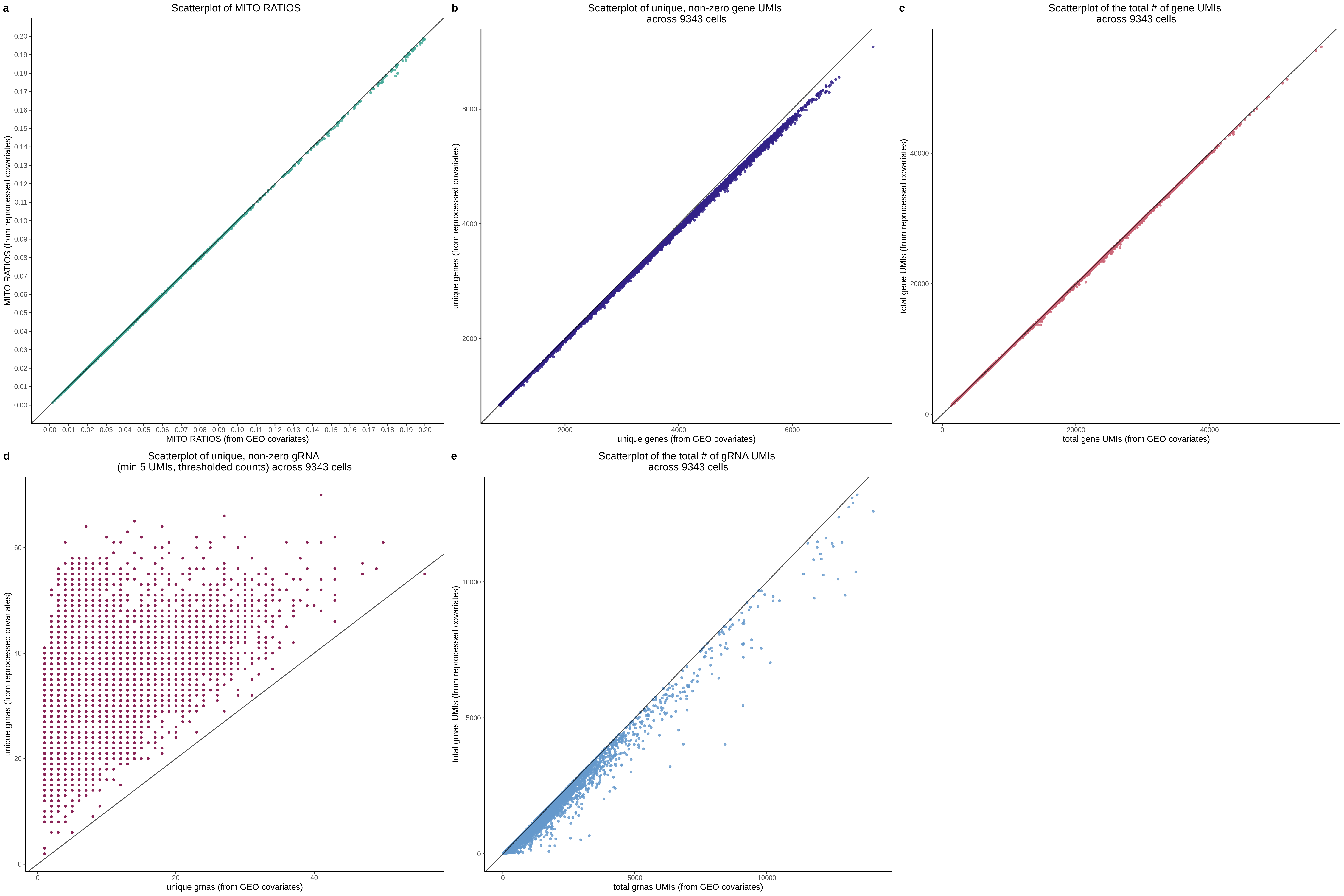
From this gridplot we can see there are two very problematic covariates; with unique gRNAs being the most extreme. I also think these show two seperate issues going on at once. For example, we can immediately see that there was a mistake in calculating the unique, nonzero gRNA UMIs. They appear uniformly larger which suggests a procedural error. This turned out to be the exact case: I was originally calculating the unique nonzero gRNAs based on the final, filtered, un-thresholded gRNA matrix. In other words, I was using the final, filtered, gRNA UMI count matrix then performing a colSums on each cell. This lead to larger than expected counts becuase cells containing a gRNA will low UMIs would still be nonzero. But Morris clearly used a covariate here calculated 1) on the thresholded gRNA matrix 2) on the unfitlered matrix. As a result, the covariate calculated in our analysis was much higher as seen on the scatterplot. Lastly, the total gRNA counts exhibit the opposite behaviour, they seem to be larger in the GEO gRNA matrix. This, along with a similar, weaker, pattern can be seen in the total gene UMIs as well, and it suggests that the covariates are actually calculated prior to filtering. Why? Becuase the sums have feature counts across genes and gRNAs that may have been potentially fitlered out/removed due to QC. This would result in the original covariates being slightly larger, which is the pattern we see in both the total gene UMIs and total gRNA UMIs. By calculating the covariates prior to filtering the matrices (cDNA + GDO) we can correct this mistake.
After correcting the issues seen above, I re-ran the paper cell barcode GEO-QC SCEPTRE run, which is a GEO-QC dedicated to running on the original paper cell barcodes (9343 cells, original genes, no custom filtering, aimed at replicating the cis results). I then replotted the covariate matrices.
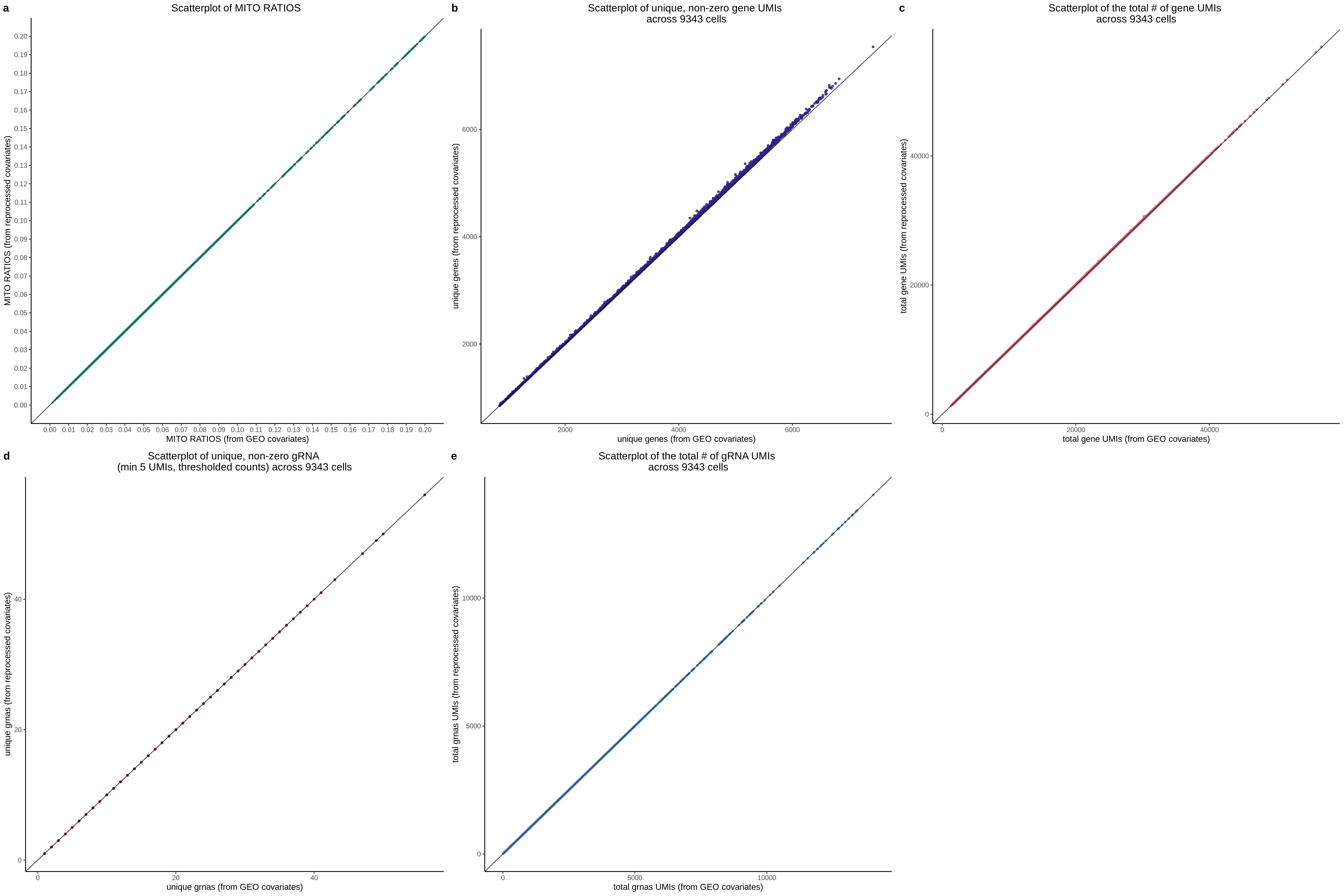
From this we can see that addressing both issue #1 and issue #2 explained above lead to an alignment of the covaraites (1:1 with the original, supplement-reported covariates per cell).
In order to evaluate if this change had an impact on the concordance of SNP (raw) p-values in the cis results, I ran the GEO-QC dedicated to the original paper barcodes and generated scatter plots between the p values seen in the SNP results reported in the supplement (1, x-axis) vs. p-values from the GEO-QC SCEPTRE run (2, y-axis). I then made a panel plot showing the original, weak concordance in PANEL A. This was actually orignally from a previous meeting, in the meeting we made this exact scatter plot, showing a large problem with the SNP p-values.
Then, from left to right, in PANEL B and in PANEL C we see two progressive changes corresponding to each issue identified above. Panel B shows the effect of correcting the unique nonzero gRNA count to be based on the thresholded matrix and Panel C shows the effect of correcting both the nonzero gRNA counts AND performing the covariate computation on the unfiltered matrices (as done by Morris). Panel C corresponds to the corrected, recalculated covariates plotted above.
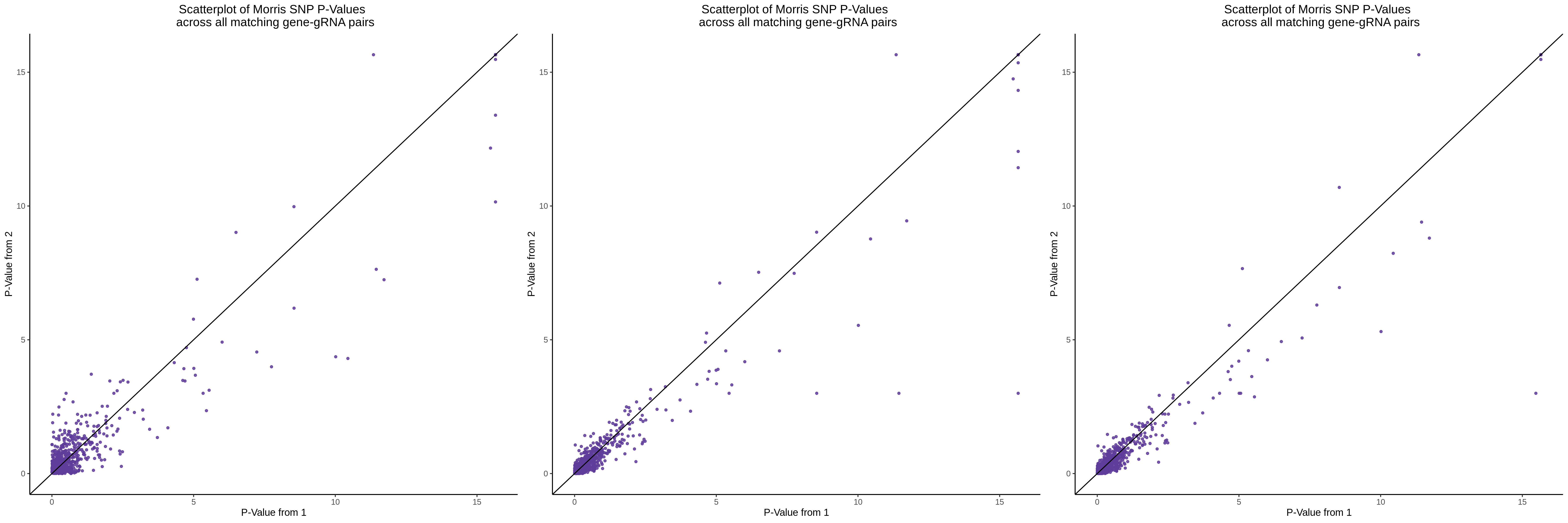
Reminder In each of the scatter plots above, the baseline reference termed “1” refers to the original results (the p value reported in the supplement) while “2” refers to the GEO-QC SCEPTRE run dedicated to original cellbarcodes.
From this I think I can conclude, to some degree, that the lack of concordance we saw in the left-most panel was likely due to the difference in covariates illustrated by the two covariate scatter-panels above. The panel on the right seems to show raw cis SNP p values that are more concordant with the original results, specifically in the moderate p-value range corresponding to log10s 2-4 (so the p value is between 0.01 - 0.0001).
Questions:
This raised questions for me:
- Why are the covariates being calculated based on unfiltered matrixes?
This is interesting to me becuase gene UMIs and gRNA UMIs for genes and gRNAs, repectively, that are not included in the final analysis (low expressed genes and low capture gRNAs) are included in the covariates. Maybe I am just not used to this. But another thing to note is the difference between the middle and right panels wherein the difference in covariates was wether or not they were calculated based on filtered or unfiltered matrices, respectively for the middle and right panels. But the difference is subtle compared to progression seen from left to middle (correcting noznero gRNA sums to be thresholded).
- Why is the GDO covariate specific to unique gRNAs based on a thresholded UMI count matrix?
8/12/2022 Notes on NTC sgRNA Library Design
The purpose of this section/notes is to elaborate and explore the library design choices used to create the sgRNAs NTC used in the Morris experiment. This was borne mostly from an interest to explore a question asked by Dr. Im during journal club regarding the exact nature of the sgRNAs being used as controls in the experiment.
- NTC taken from the GECKO V2 library (NTC labrary)
- Sanjana Lab
- manual: “GUIDES: sgRNA design for LOF screens”
- bioxRV
- NTC definition: sgRNA designed NOT to target in the respective genome (ie Homo sapiens)
- design notes:
- thousands of random 20mer sequences (10K)
- aligned to target genome (ie Homo sapiens) with 0,1,2,3 mismatches
- done in bowtie short read aligner
- final sgRNAs added to the GECKO V2 library are nontargetting
to the human genome with up to 3 mismatches
- the wording on this definition is tricky since we are actually selecting for those 20kmer sequnces that can tolerate 3 mismatches and still not align to human reference
- A G-Score is calculated for each random 20mer seq. to evaluate its
off target capacity
- G-Score integrates cutting frequency determination in order to estimate the rate at which sgRNA can cut off an certain off target site
- based on experimental data from ~10K sgRNAs with mismatches, dels, and insertions
- general idea: is to select sgRNAs that dont align to target genome with up to 3 mismatches
- we remove sgRNAs from the pool that align, keep those that dont with up to 3 mismatches
- The end result: GECKO V2 library with 1,000 NTC sgRNAs (out of 10K random candidate NTCs)
8/10/2022 gRNA UMI Scatter Plots
The goal is to compare the Morris gRNA matrix in GEO against the re-processed Kallisto bustools gRNA matrix of the same data, subset to the 9343 cells used in the orginal analysis. We want to answer the question: is there a significant difference between the two same gRNA matrixes? This is important because these matrixes are used, respectively, for the GEO-QC and QC RUNS below.
Our general expectation is that the two matrixes are near identical or at least contain concordant UMI counts between the identical cell barcodes in each matrix. We expect this becuase both gRNA matrixes were generated through the Kallisto-Bustools KITE workflow. Briefly, this workflow consists of two steps: 1) making a novel fasta reference for each possible gRNA sequence (hammiing distance = 1bp) 2) counting appearences of sequences from (1).
Both matrixes contain counts for 210 Morris gRNAs, but differ in the total amount of cells (unfiltered) lighty. The GEO gRNA matrix size is: 210 X 137.3K and the re-processed matrix size is: 210 X 137K, a ~300 cell difference. We subset the gRNA matrixes to the original analysis cells, using their cell barcodes reported in the supplement.
In order to explore the comparison, we plot scatter plots and histograms showing the distribution of UMI counts per gRNA across all 210 gRNAs subset to 9343 cells used in the original analysis. Below we look at a few specific examples:
Here we look at CD55-1, a PTC gRNA targetting the ~TSS of the CD55 gene.
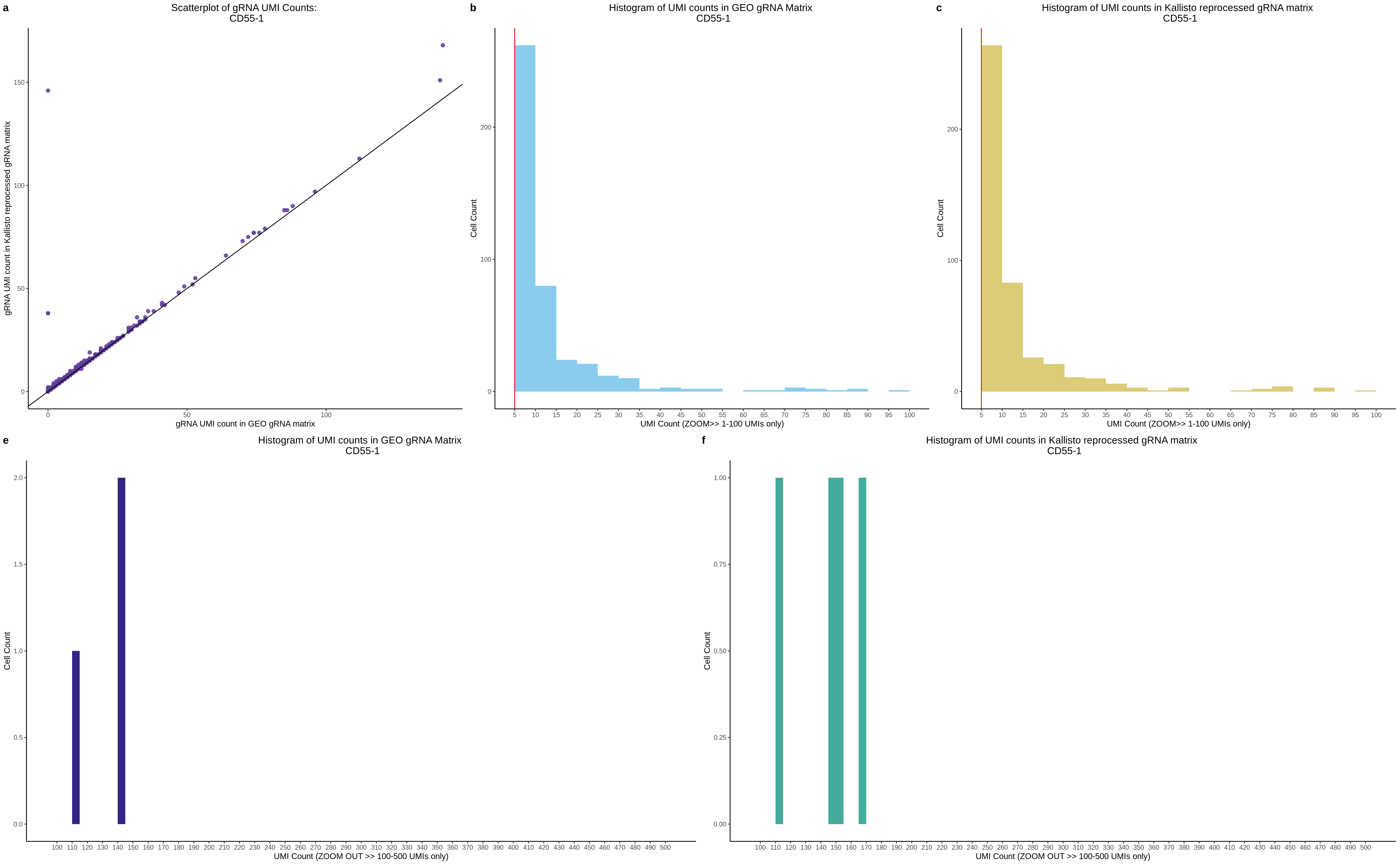
Here we see that the UMI counts between matrixes are strongly concordant with most of the 9343 cells containing between 0-50 UMIs for this gRNA (histogram 0-100 clearly shows the bulk of the cells containing UMIs greater than 5).
Here we look at NTC-6, a NTC gRNA.
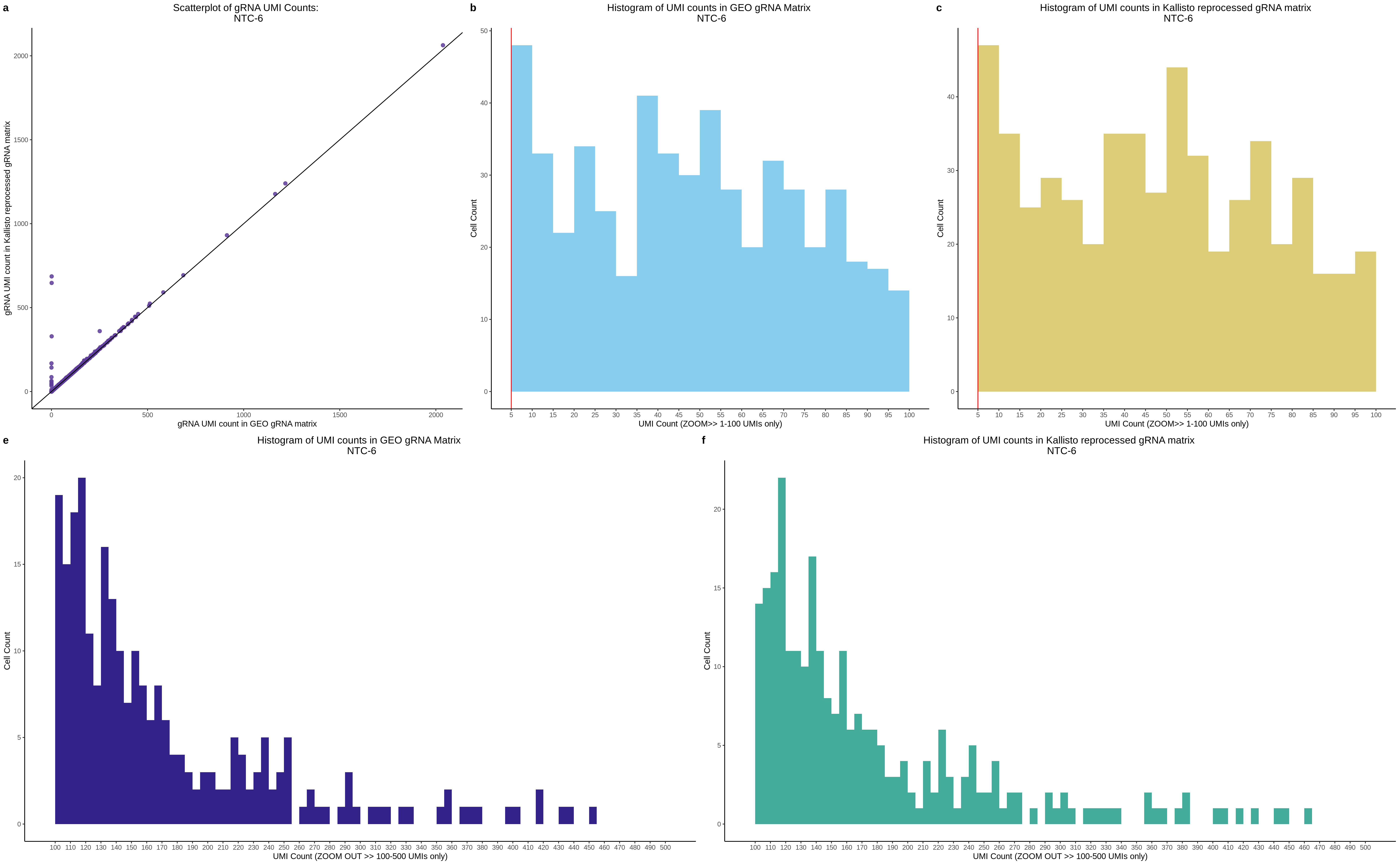
Here we look at NTC-10, a NTC gRNA that is tested the most (~10K pairs) in the cis analysis.
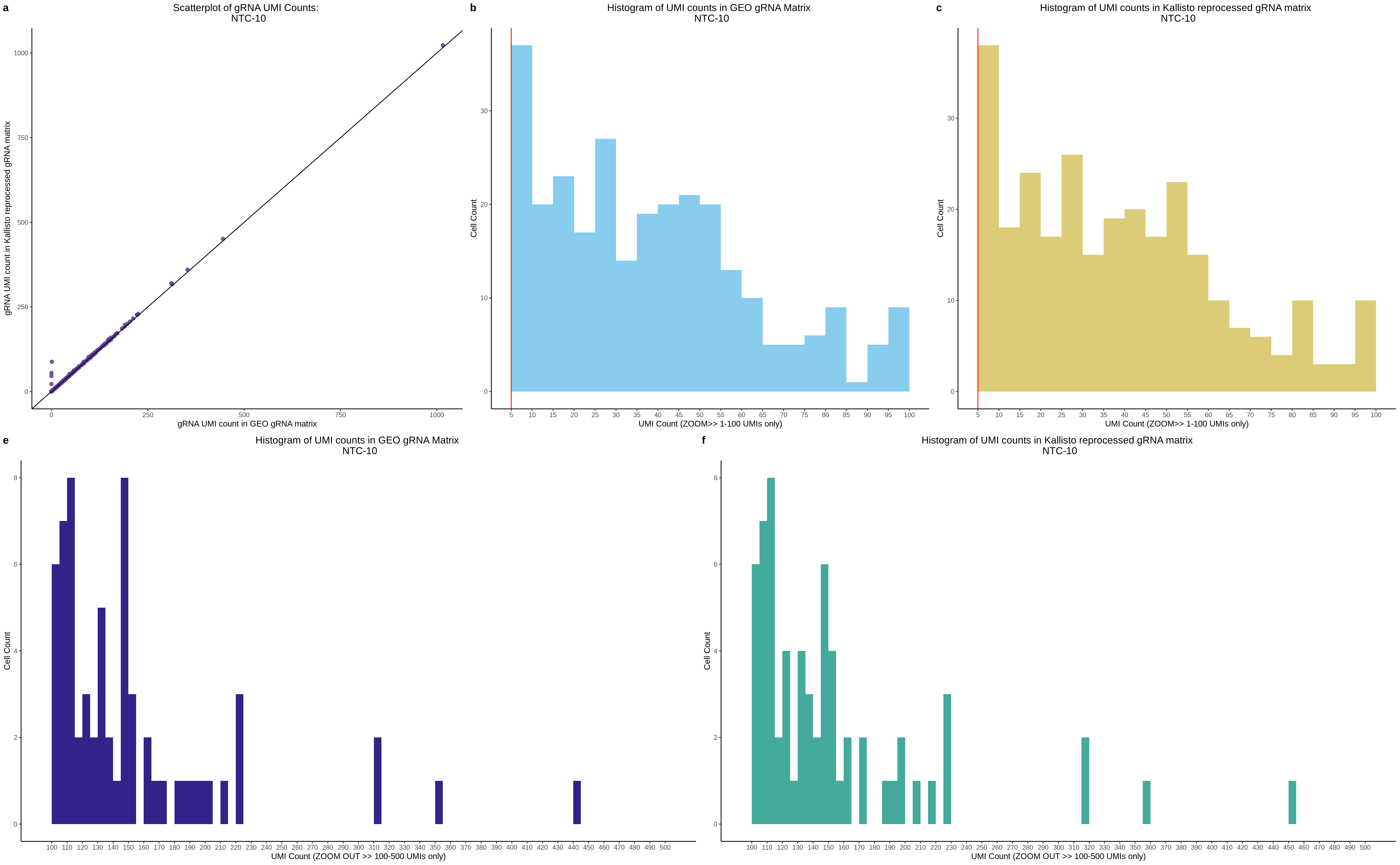
Here we look at **SNP-76-2*
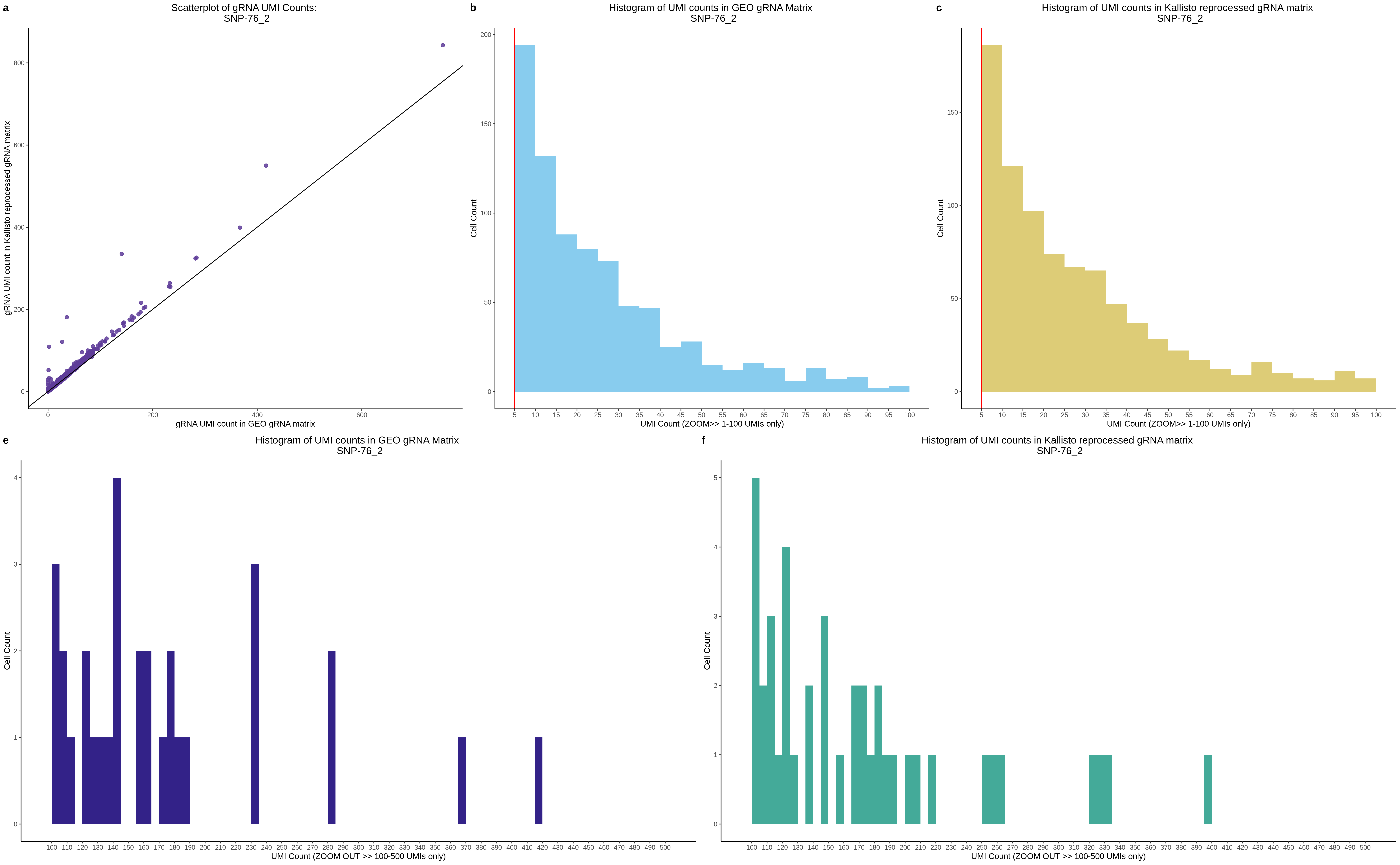
Here we look at **SNP-76-1*
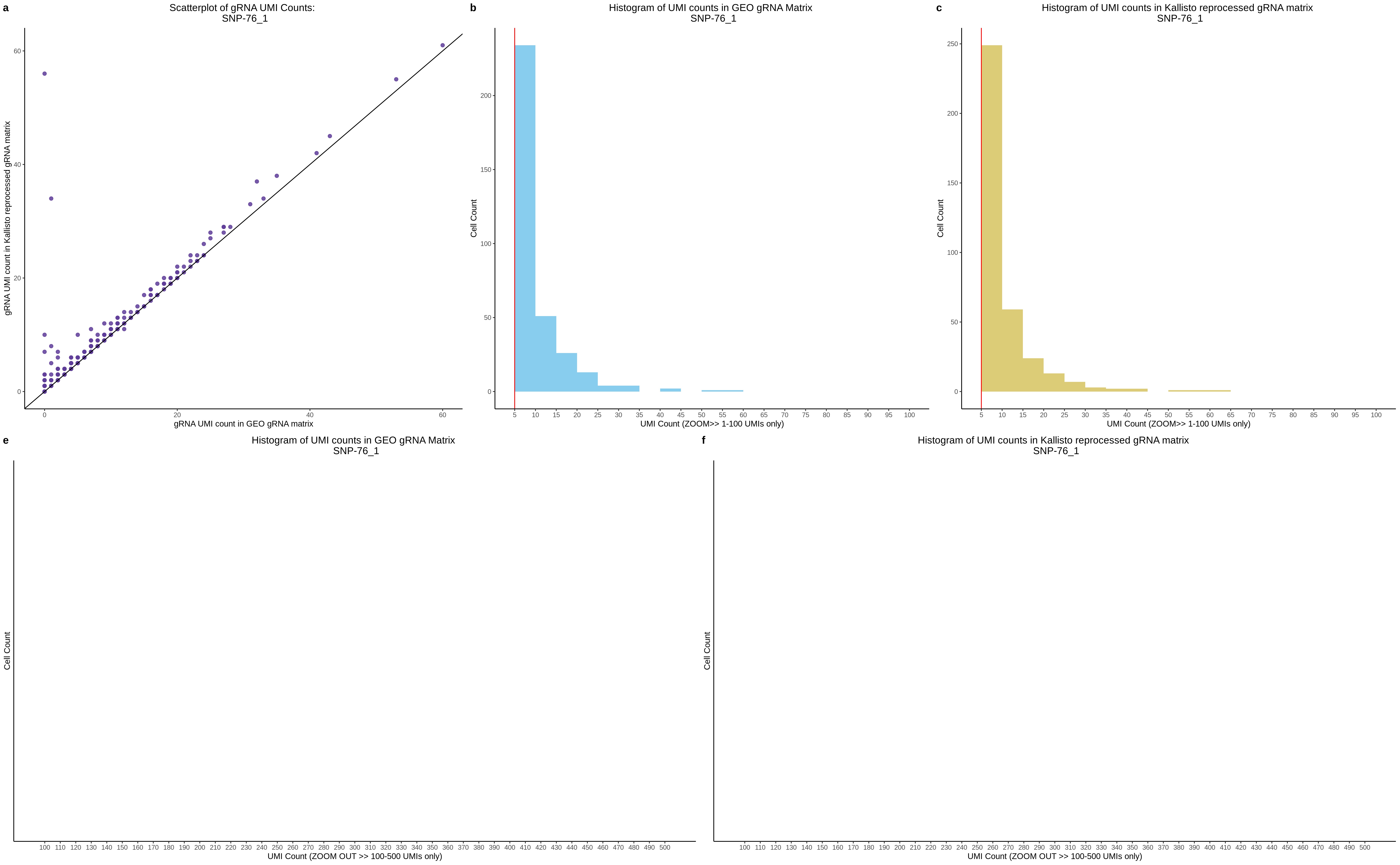
We can see based on these two gRNA that sometimes a gRNA is clearly better in terms of the number of cells that gRNA is later detected in. But in both cases the cell-specific UMI count was mostly concordant despite on gRNA being clearly better in the context of the experiment.
This pattern is Not always the case, some gRNA appear to be very different between the two matrixes.
For example, lets look at one of the problem gRNA we identified earlier again:
SNP-44-2
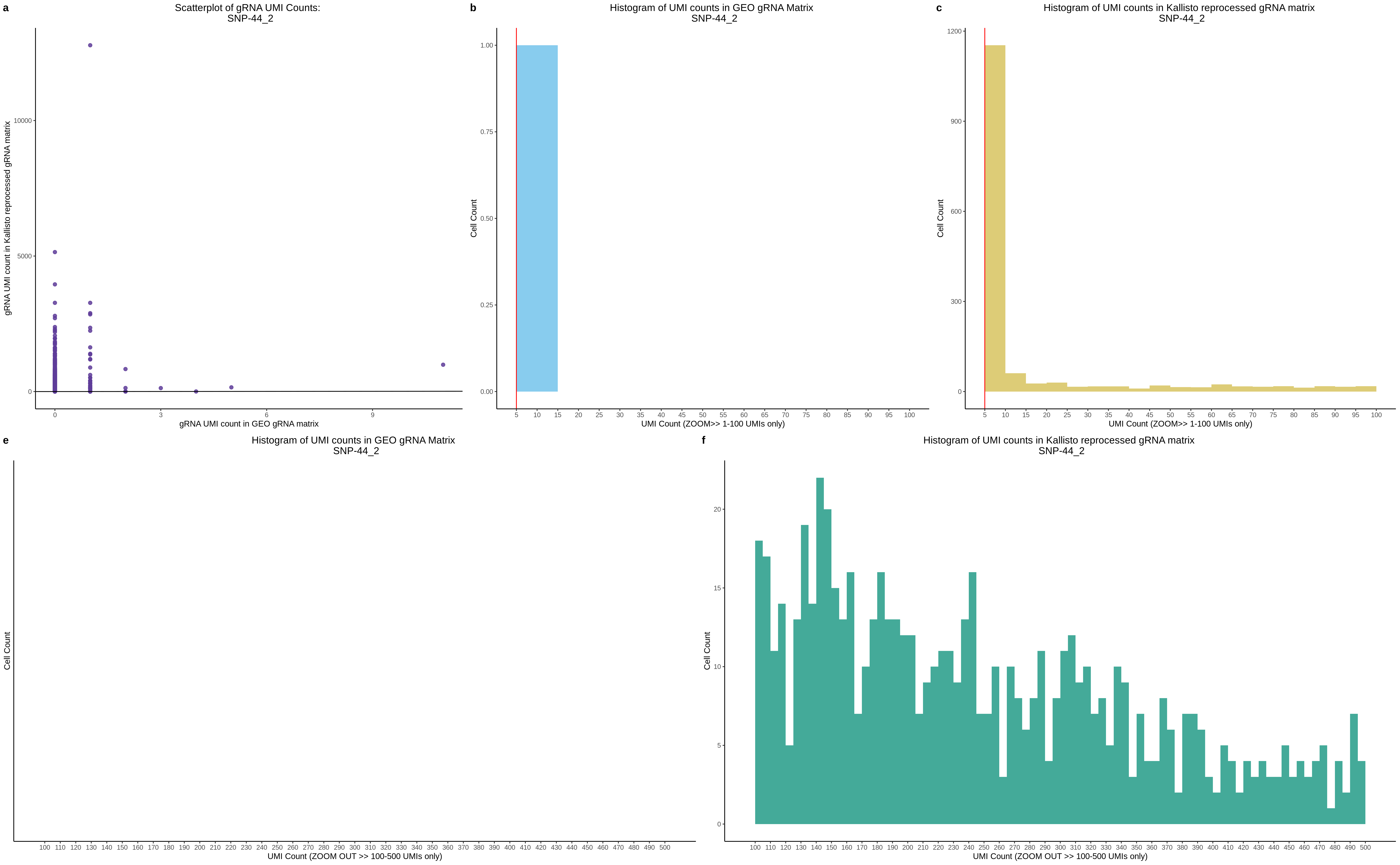
In another case, vice versa behaviour, the GEO matrix seems to contain UMI counts while the reprocessed matrix contains almost no cells with these two PTC gRNA targetting the same PTC gene.
HSPA8-2 and HSPA8-1
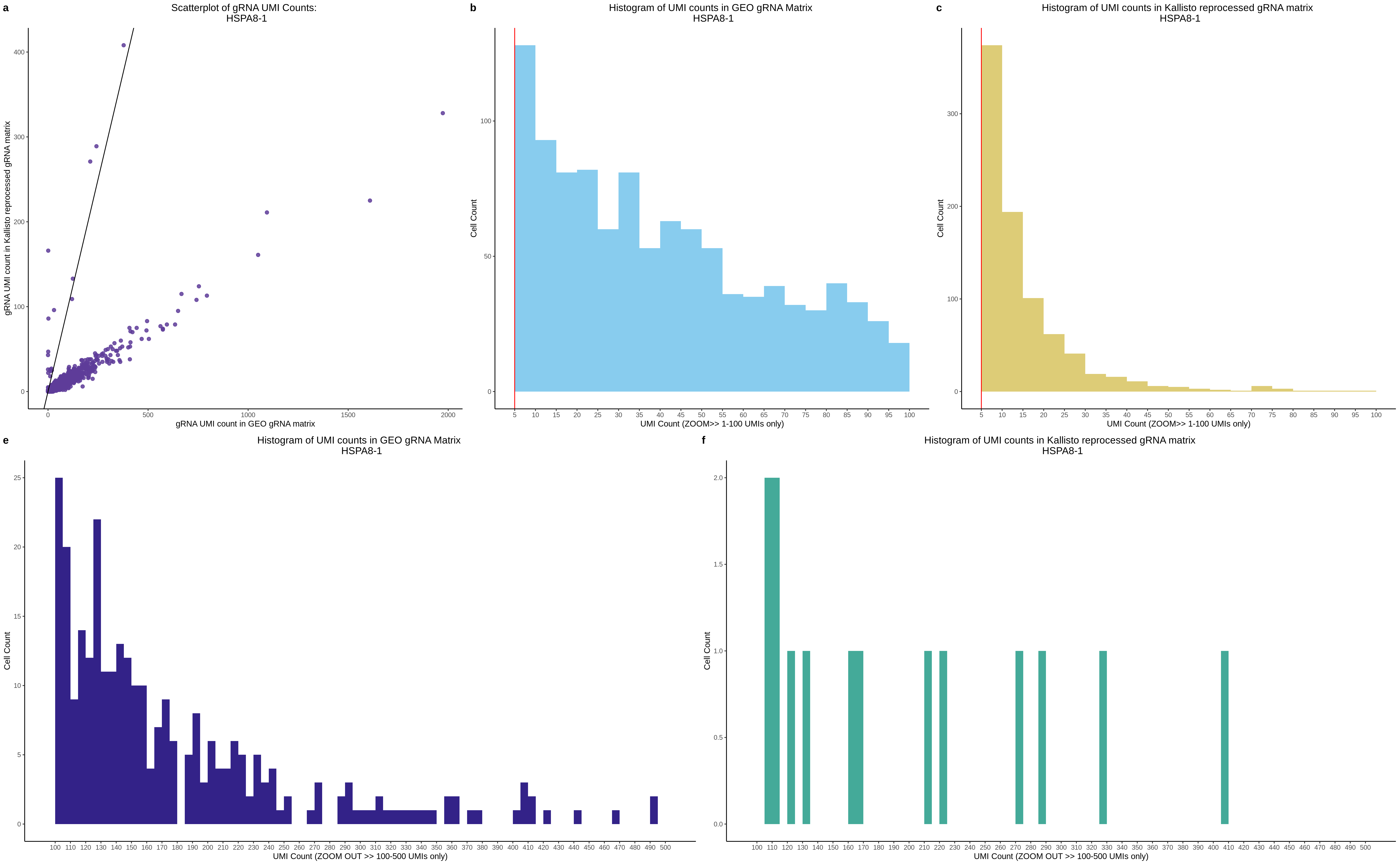
8/10/2022 Overlap of cis Morris results
The goal here is look closer into various QC methods and their affect on overlap in terms of signal (significant pairs). Briefly, the Morris data was either taken from GEO (GEO-QC) or reprocessed from raw data (QC) and then the orginal cis pairs were tested for association with the expectation that there will be a strong overlap in signal and concordant raw p values amongnst cis signals.
Summary of run analysis:
| RUN | cell detectability threshold | min unique UMIs | min total UMIs | dataset desc. |
|---|---|---|---|---|
| GEO original | ~5% | 850 | X | (original pairs + original results as reported in manuscript/supplement) |
| GEO paper QC | X | X | X | original pairs + data QC: subset to cell barcodes/genes/gRNAs reported in results |
| GEO-QC1 | 0.5% | 1200 | 1200 | original pairs + original NTCs |
| GEO-QC2 | 5% | 1200 | 1200 | original pairs + original NTCs |
| GEO-QC3 | 5% | 1200 | 1200 | cis pairs based on 500 kb distance + all NTCs |
| QC1 | 0.5% | 1200 | 1200 | original pairs + original NTCs |
| QC2 | 5% | 1200 | 1200 | original pairs + original NTCs |
| QC3 | 5% | 1200 | 1200 | cis pairs based on 500 kb distance + all NTCs |
Its important to point out that the first two RUNS are control-esque. The first run entered is simply the results reported in the supplement and QC metrics taken from the paper (850). The second RUN in the table is aimed at re-creating the paper results as accurately as possible by 1) No new QC 2) original pairs. The idea here is that when we take data from GEO and rerun the orginal cis pairs we should get nearly identical p values and equal signals since its as close to the manuscript results as possible.
The other RUNS are seperated into GEO-QC or QC categories to indicate where the data is sourced from and the table further idicates which QC thresholds were used on those cis SCEPTRE runs.
Imporant note: in all of these plots below results: 1 always corresponds to the original SCEPTRE results. This would be the first entry in the table above (original pairs, original results from supplement).
Original vs GEO-QC2
Here we compare the original results to the results from GEO-QC2. In both cases, FDR and Bonferroni corrections were applied to BOTH the SNP and PTC pairs, becuase there are only a few PTC pairs that we test for association (11).
Overlap of PTC signals (FDR, Bonferroni)


Overlap of SNP signals (FDR, Bonferroni)
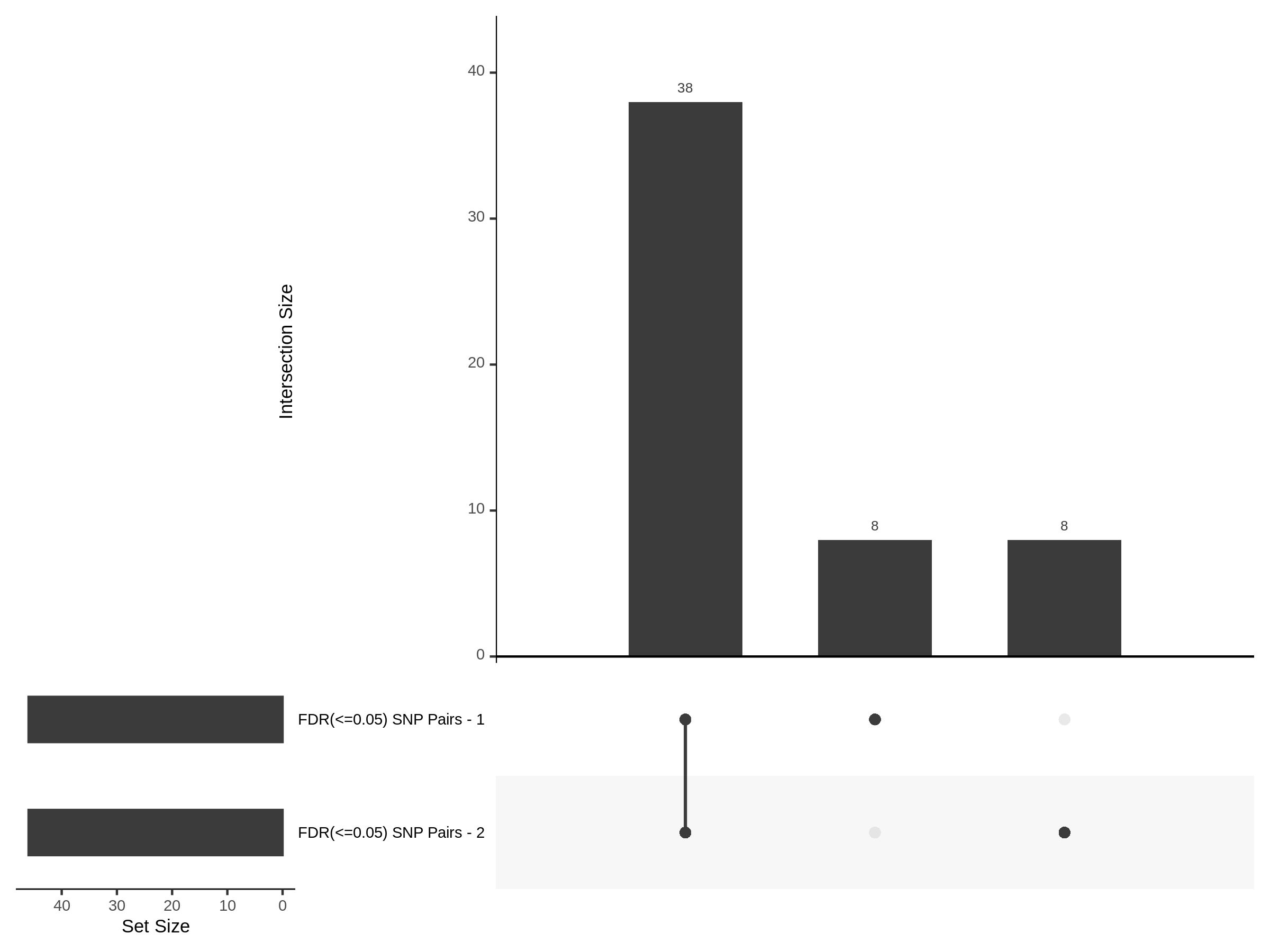

Scatterplot of PTC signals:

Original vs QC2
Overlap of PTC signals (FDR, Bonferroni)


Overlap of SNP signals (FDR, Bonferroni)
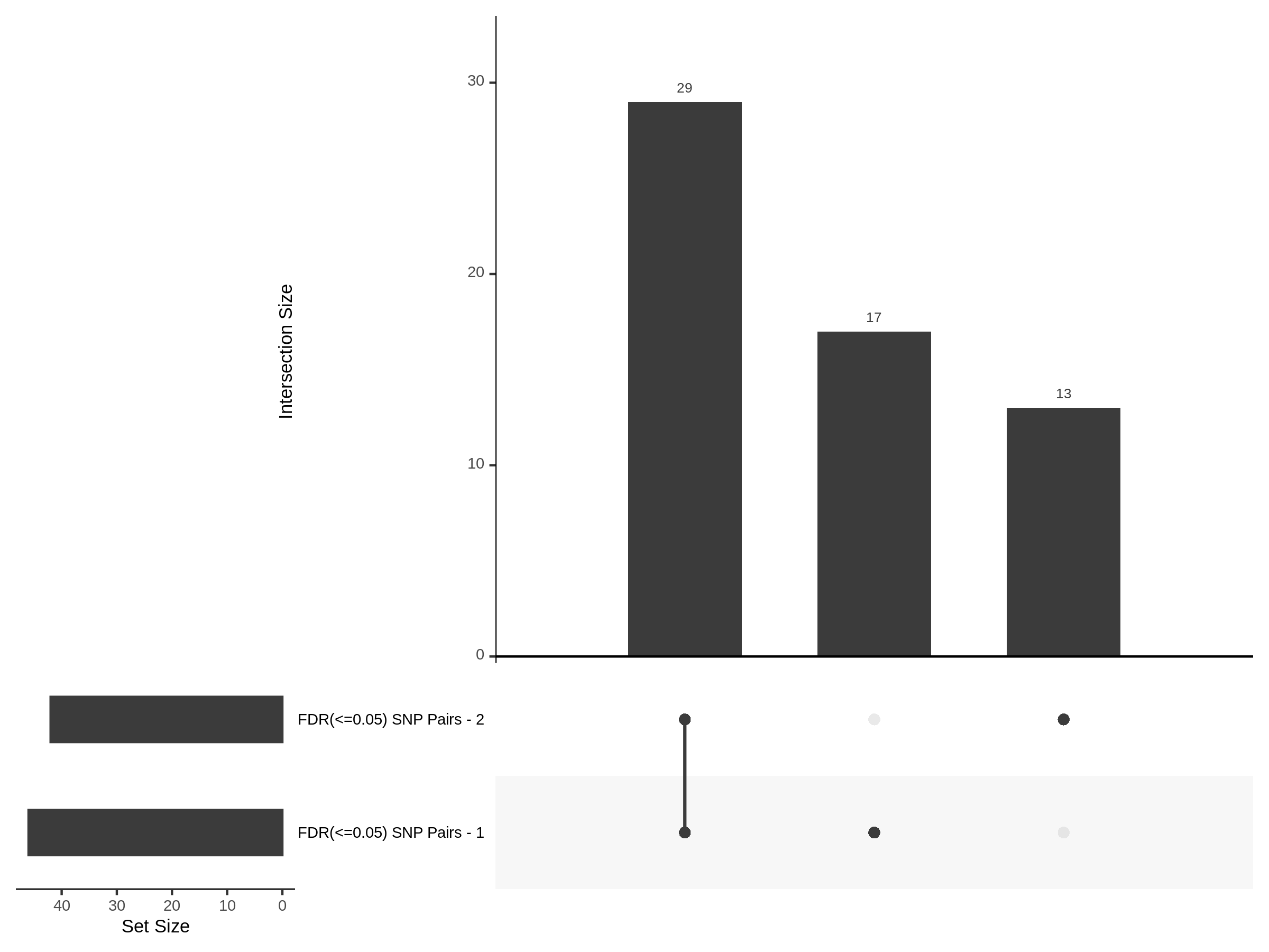

Scatterplot of PTC signals:
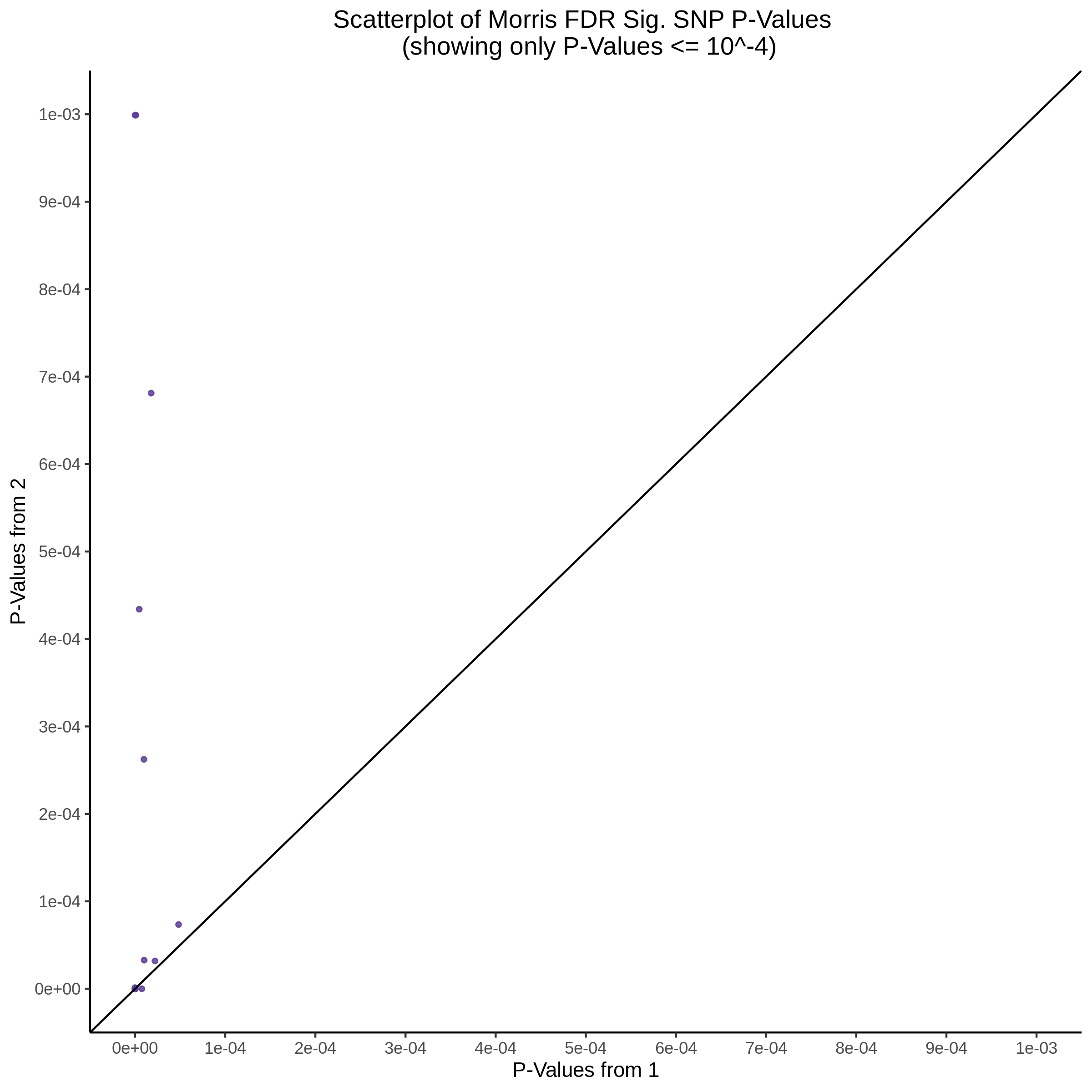
Original vs GEO-QC1
Overlap of PTC signals (FDR, Bonferroni)

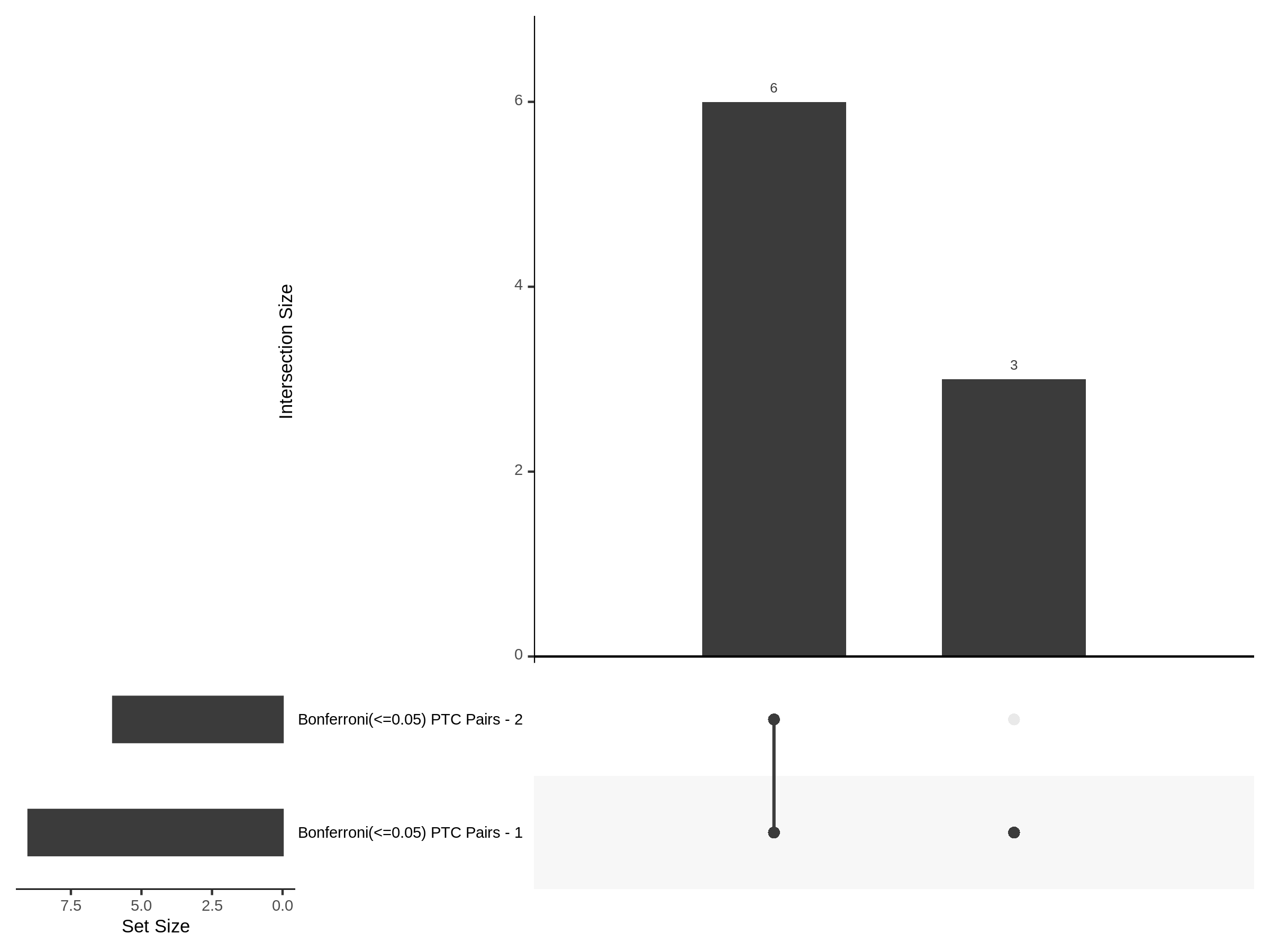
Overlap of SNP signals (FDR, Bonferroni)
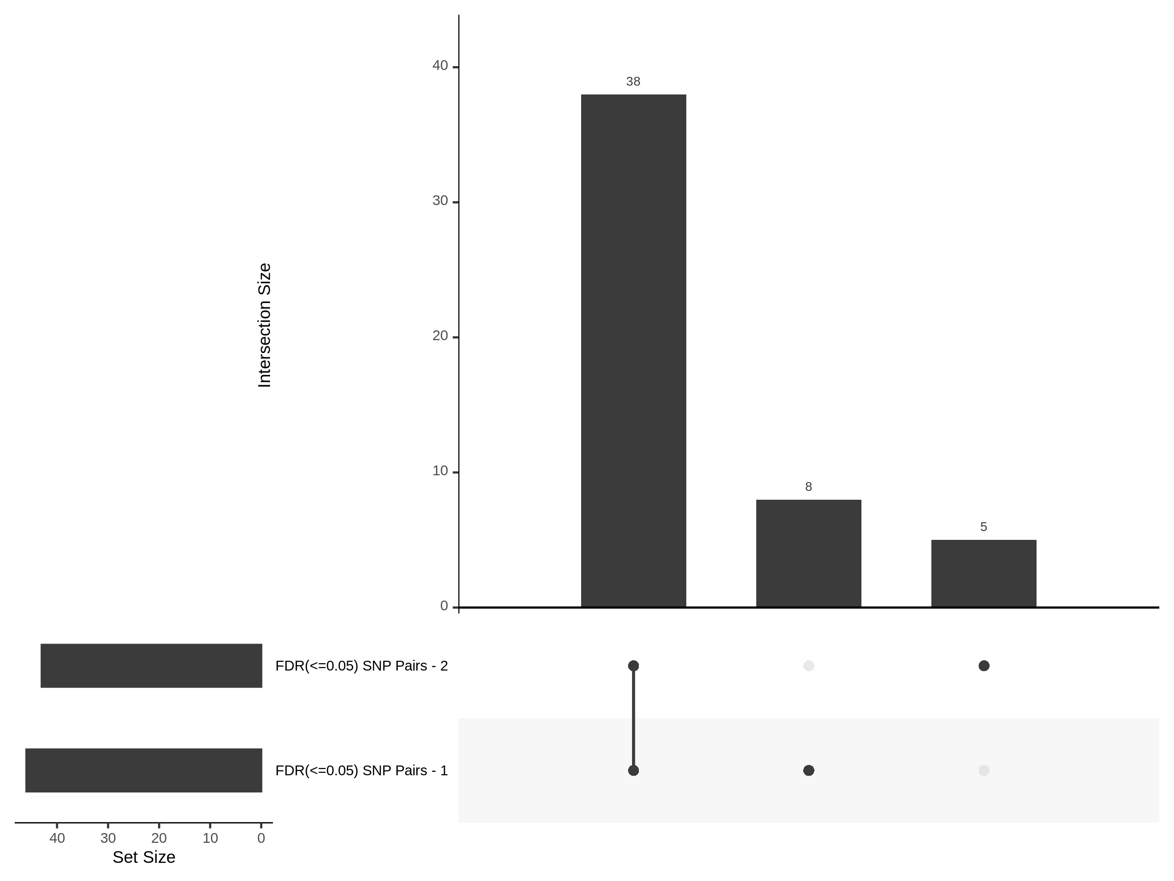
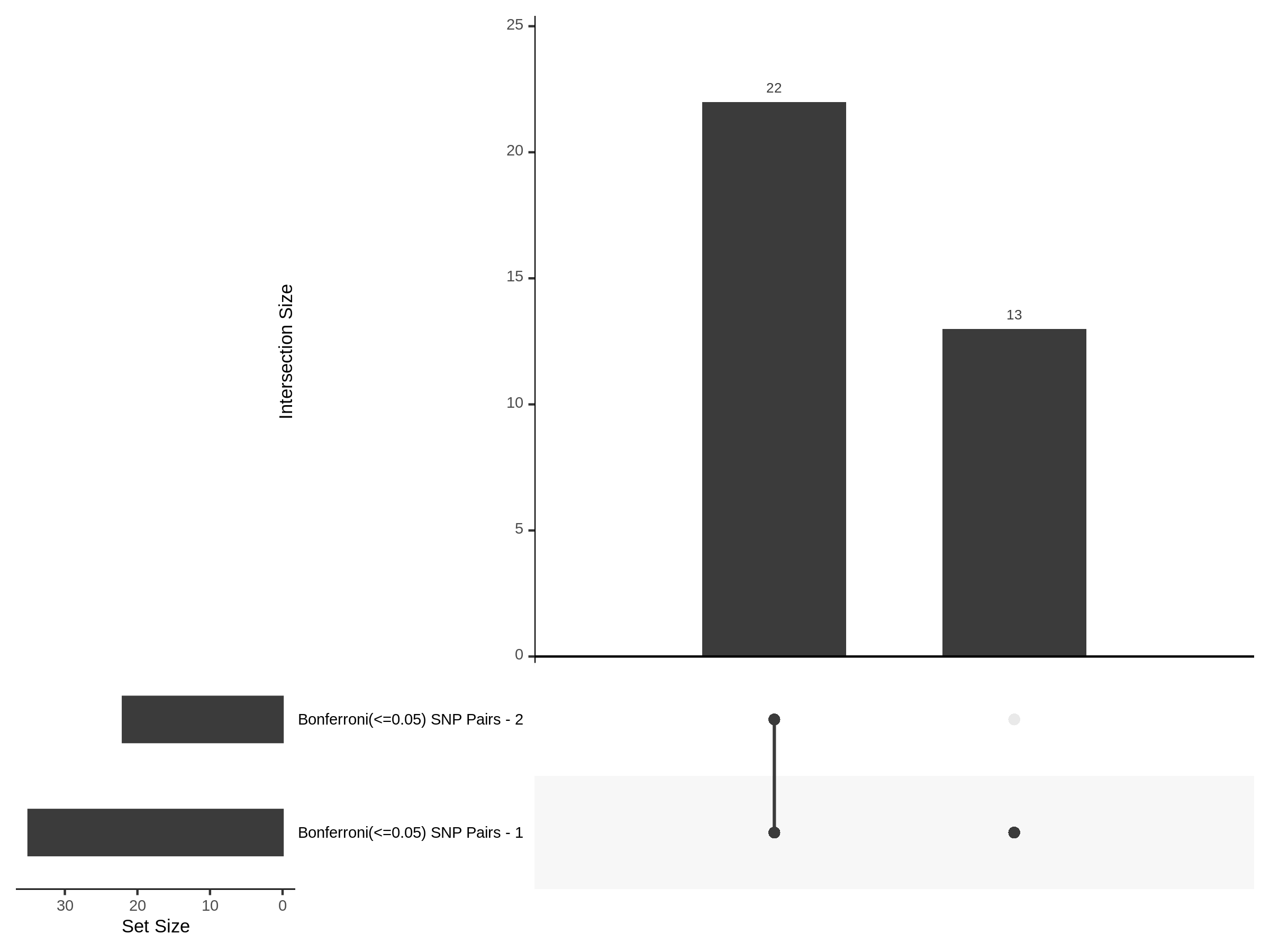
Scatterplot of PTC signals:

Original vs QC1
Overlap of PTC signals (FDR, Bonferroni)

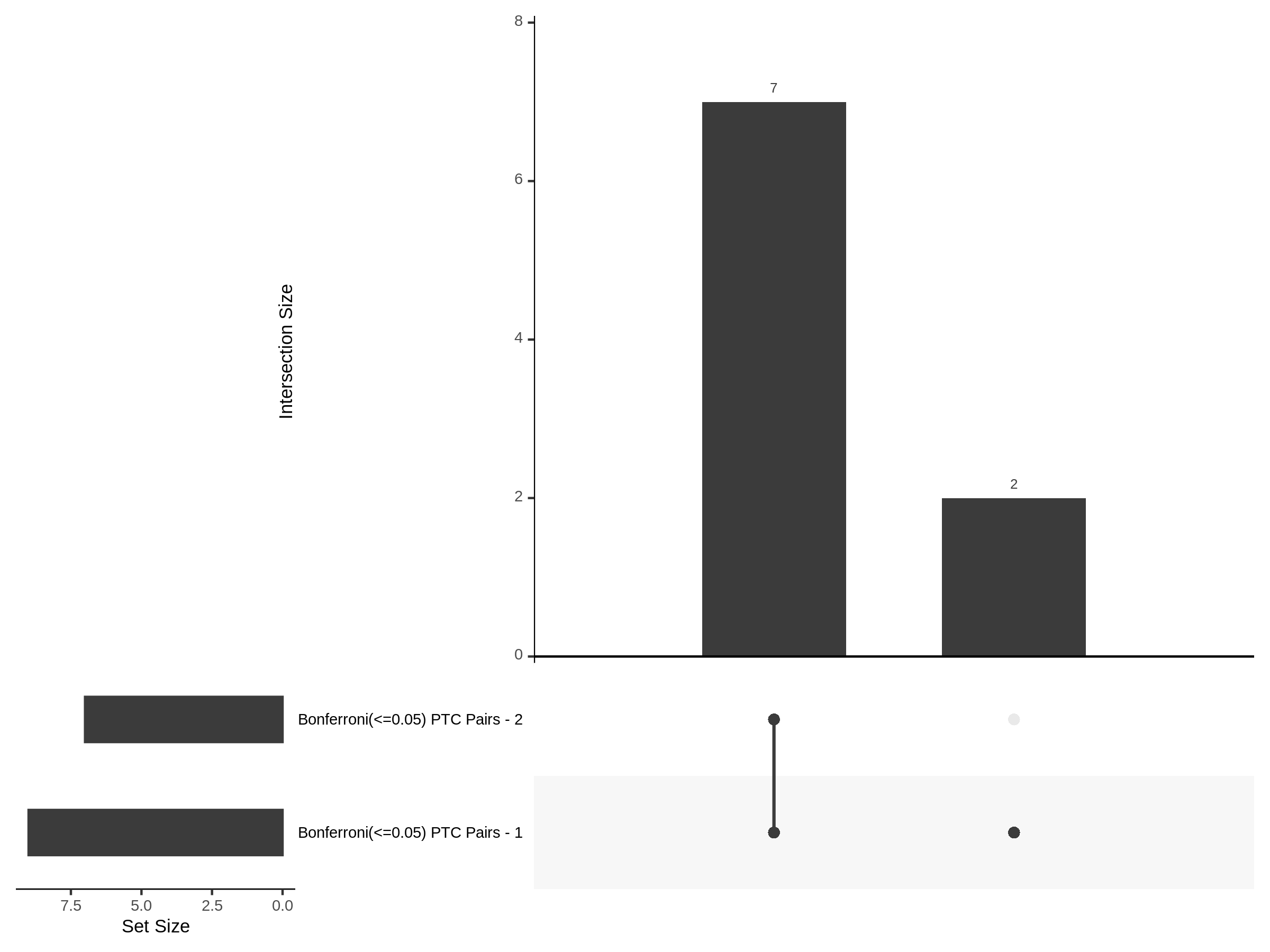
Overlap of SNP signals (FDR, Bonferroni)
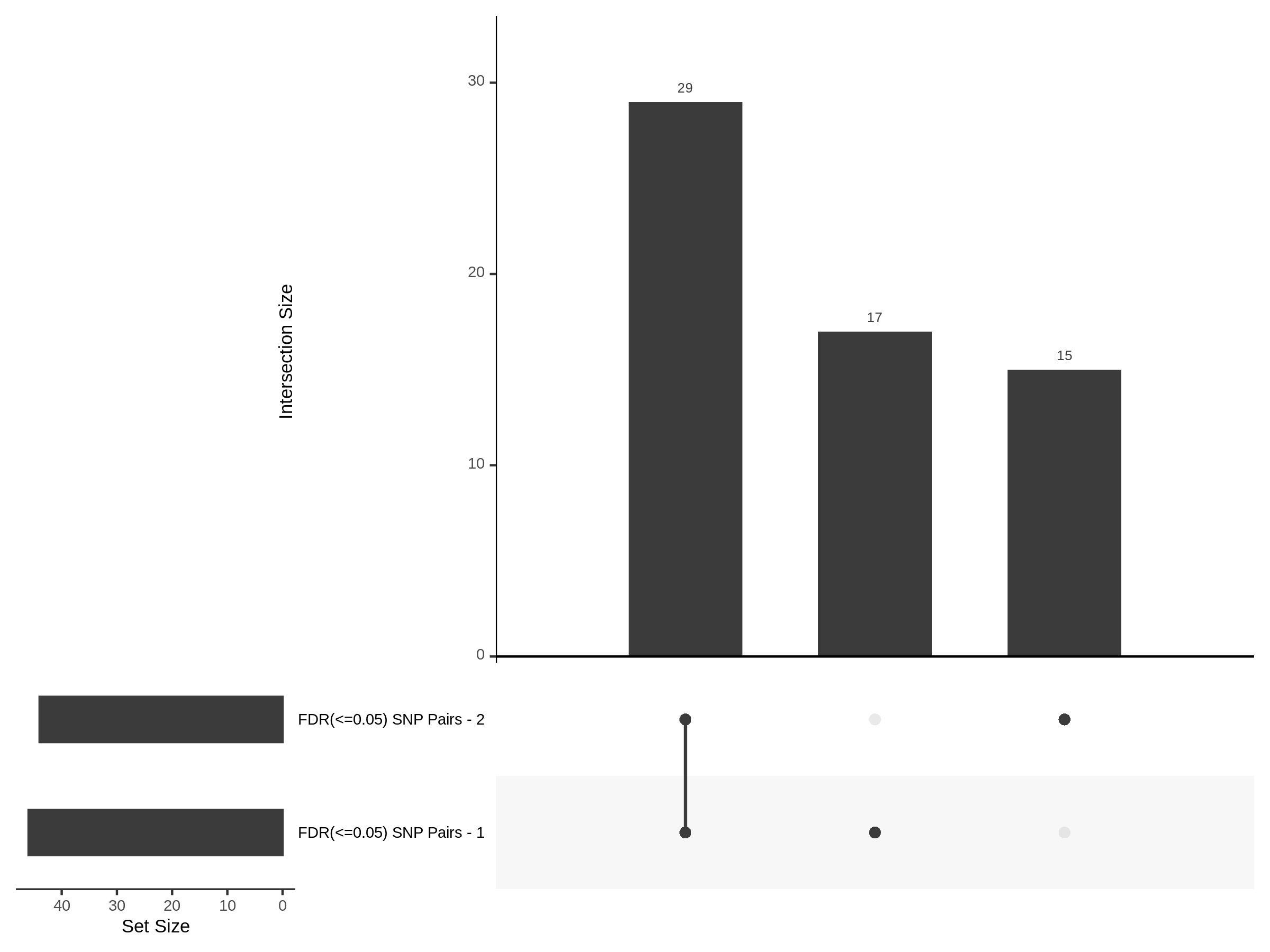
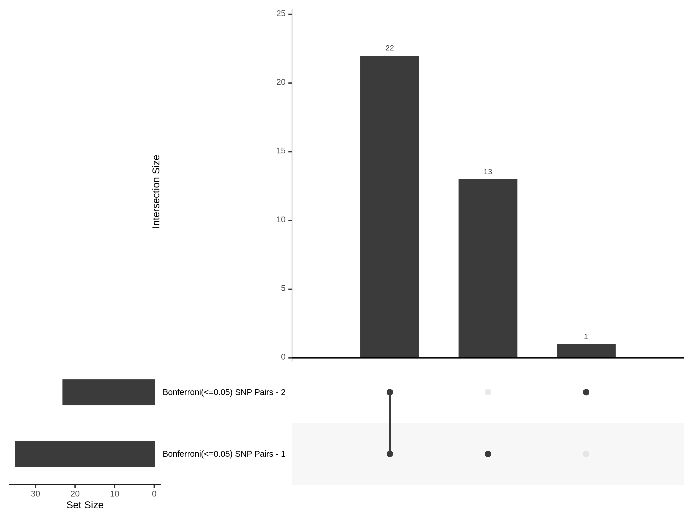
Scatterplot of PTC signals:

Original vs GEO-QC3
Overlap of PTC signals (FDR, Bonferroni)
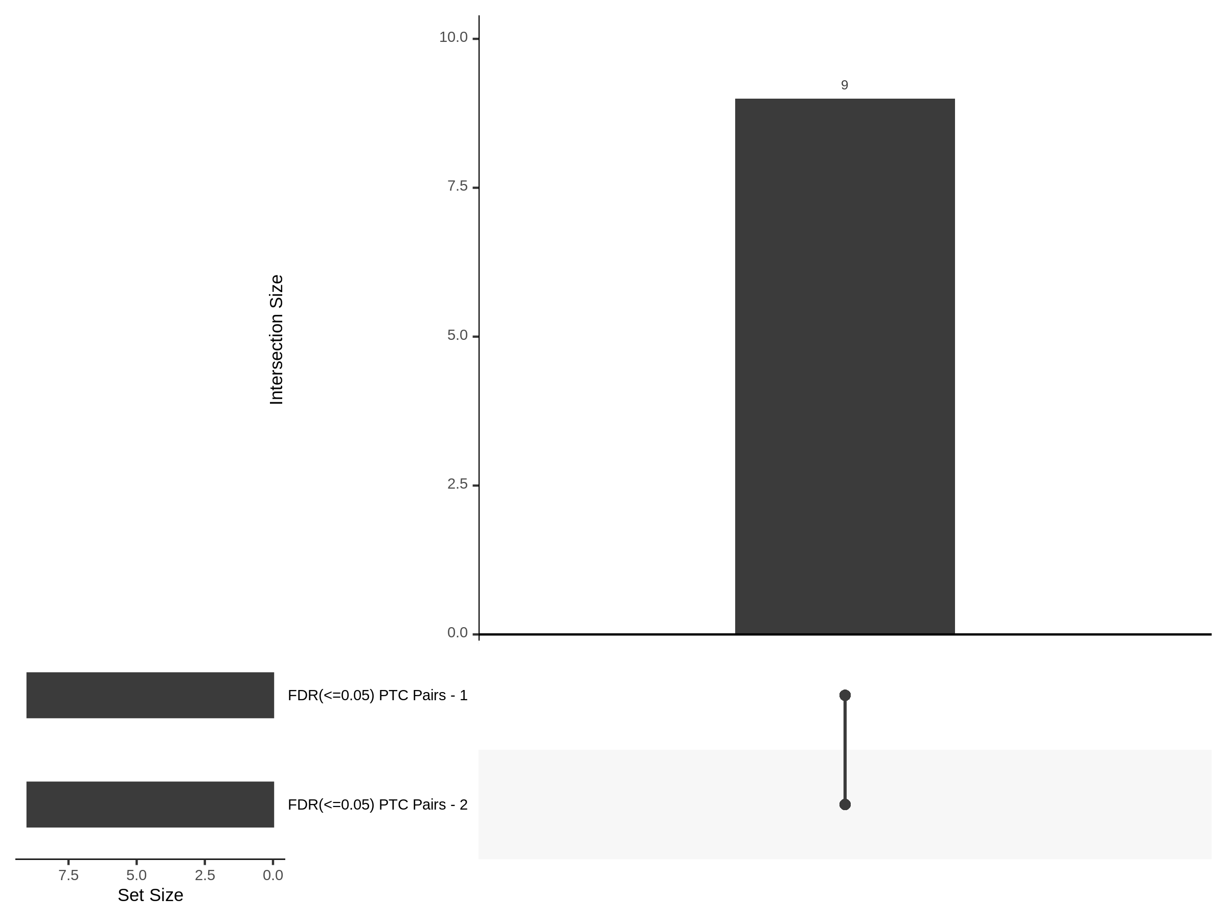

Overlap of SNP signals (FDR, Bonferroni)
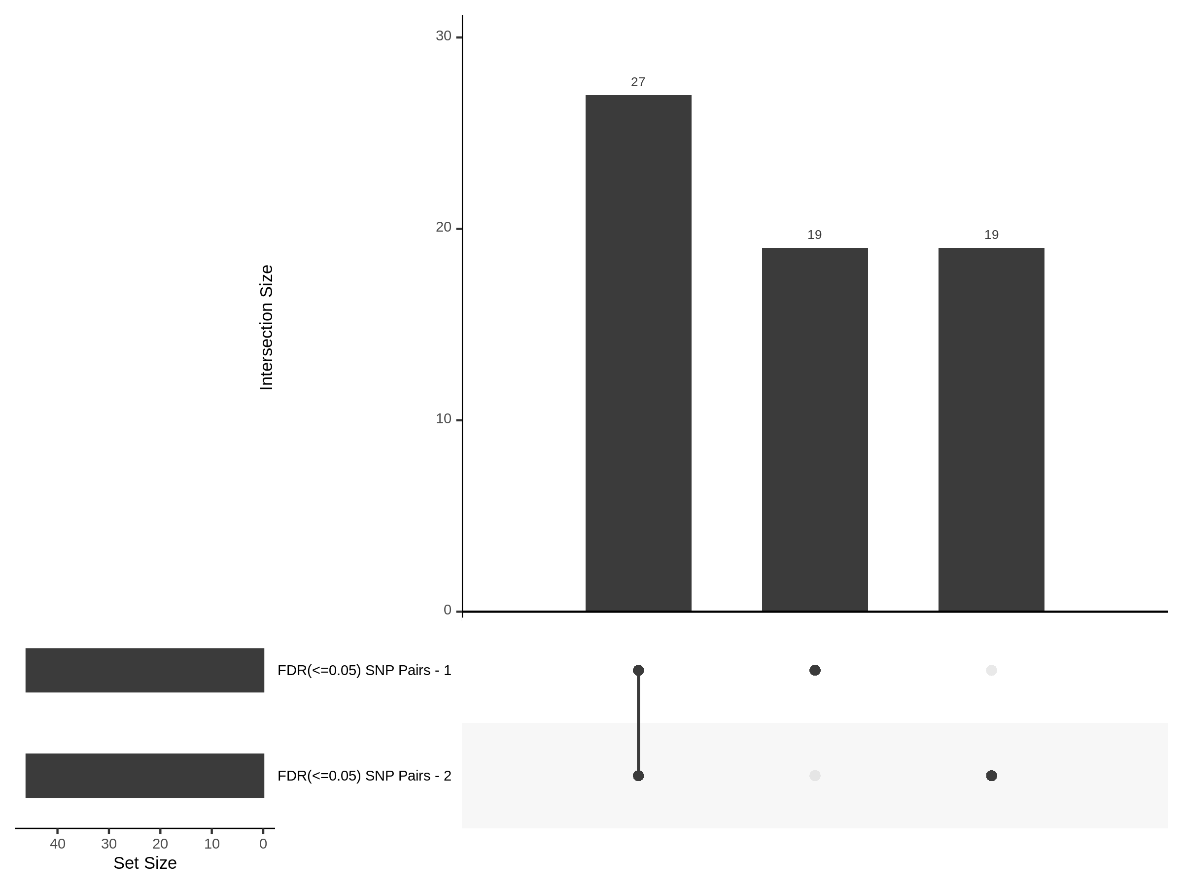
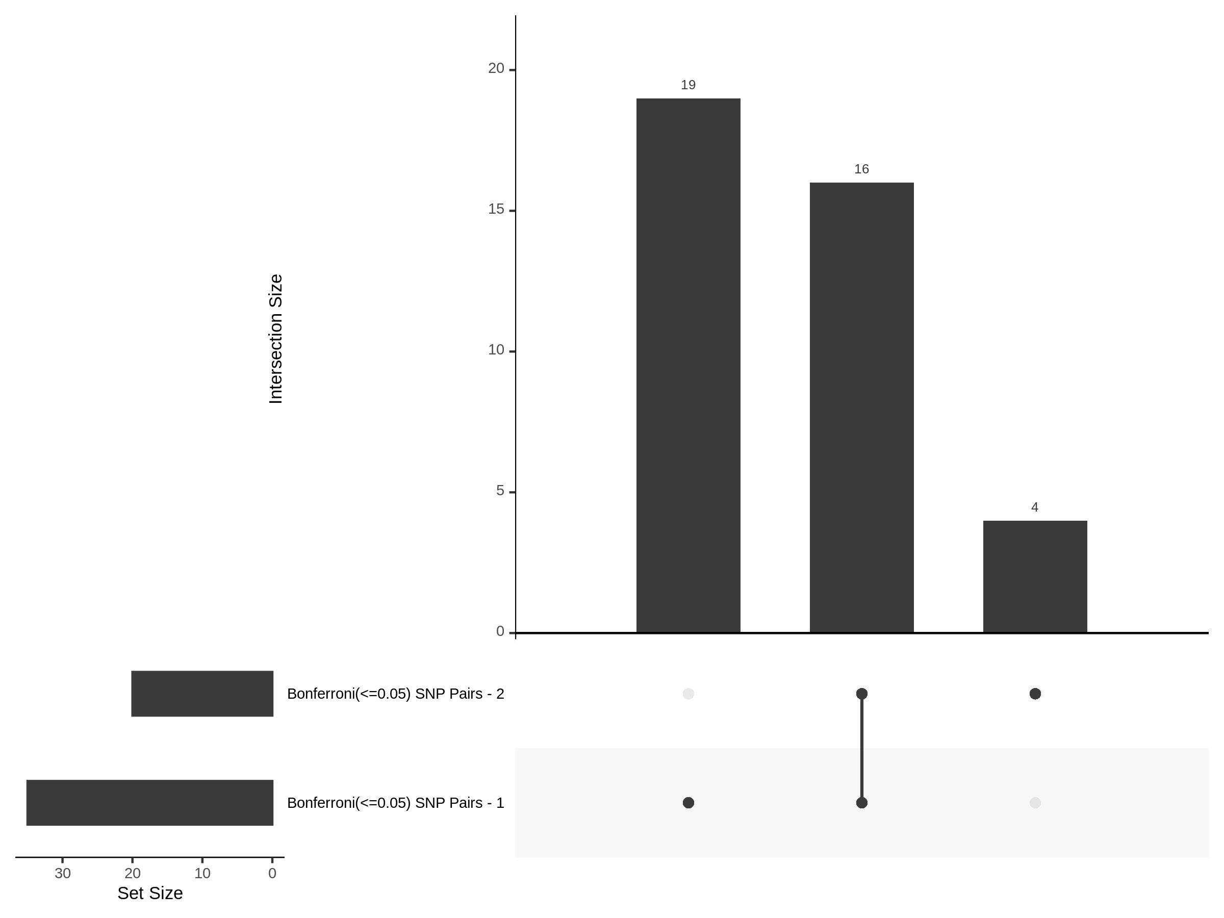
Scatterplot of PTC signals:

Original vs QC1
Overlap of PTC signals (FDR, Bonferroni)


Overlap of SNP signals (FDR, Bonferroni)
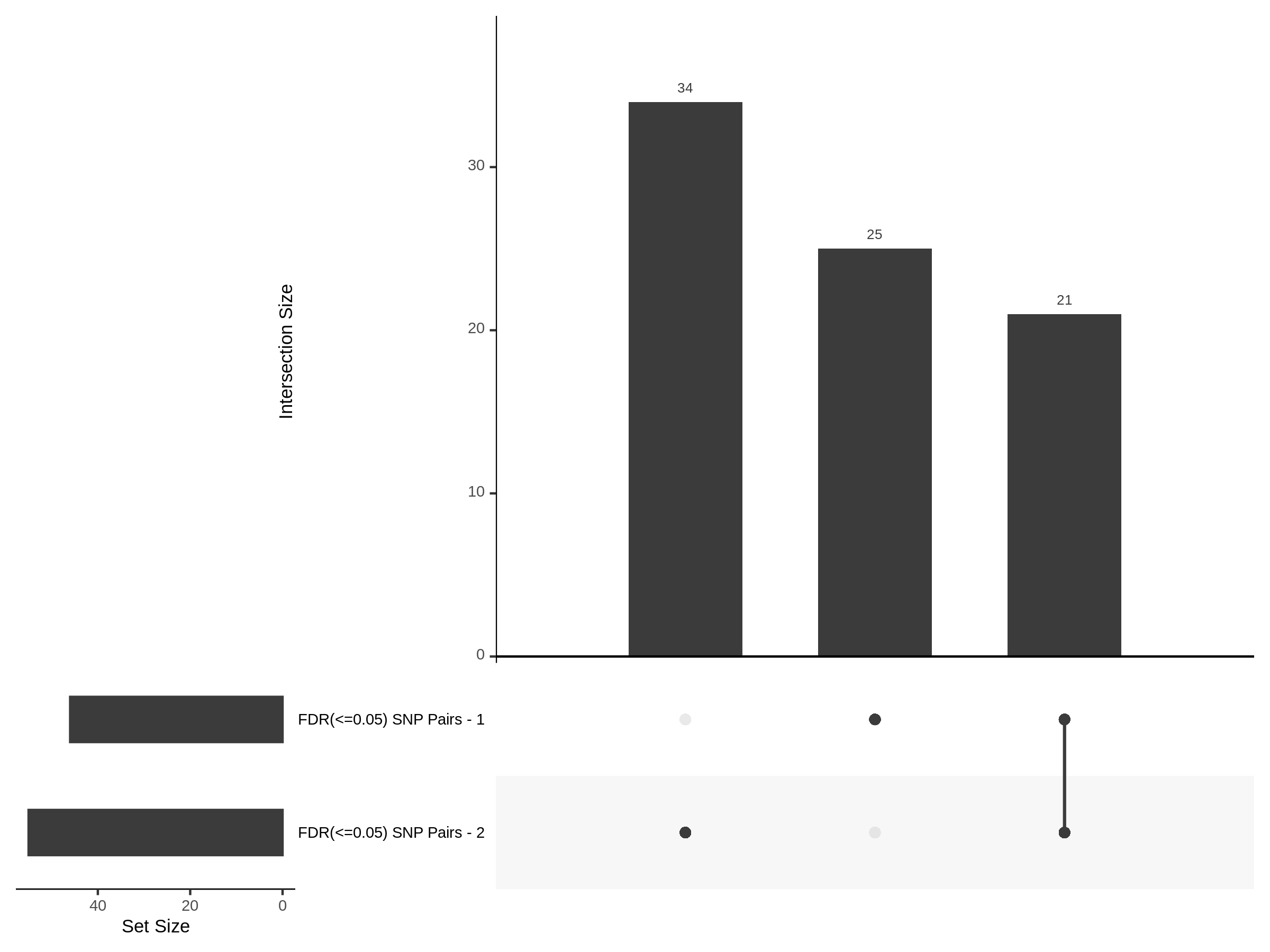
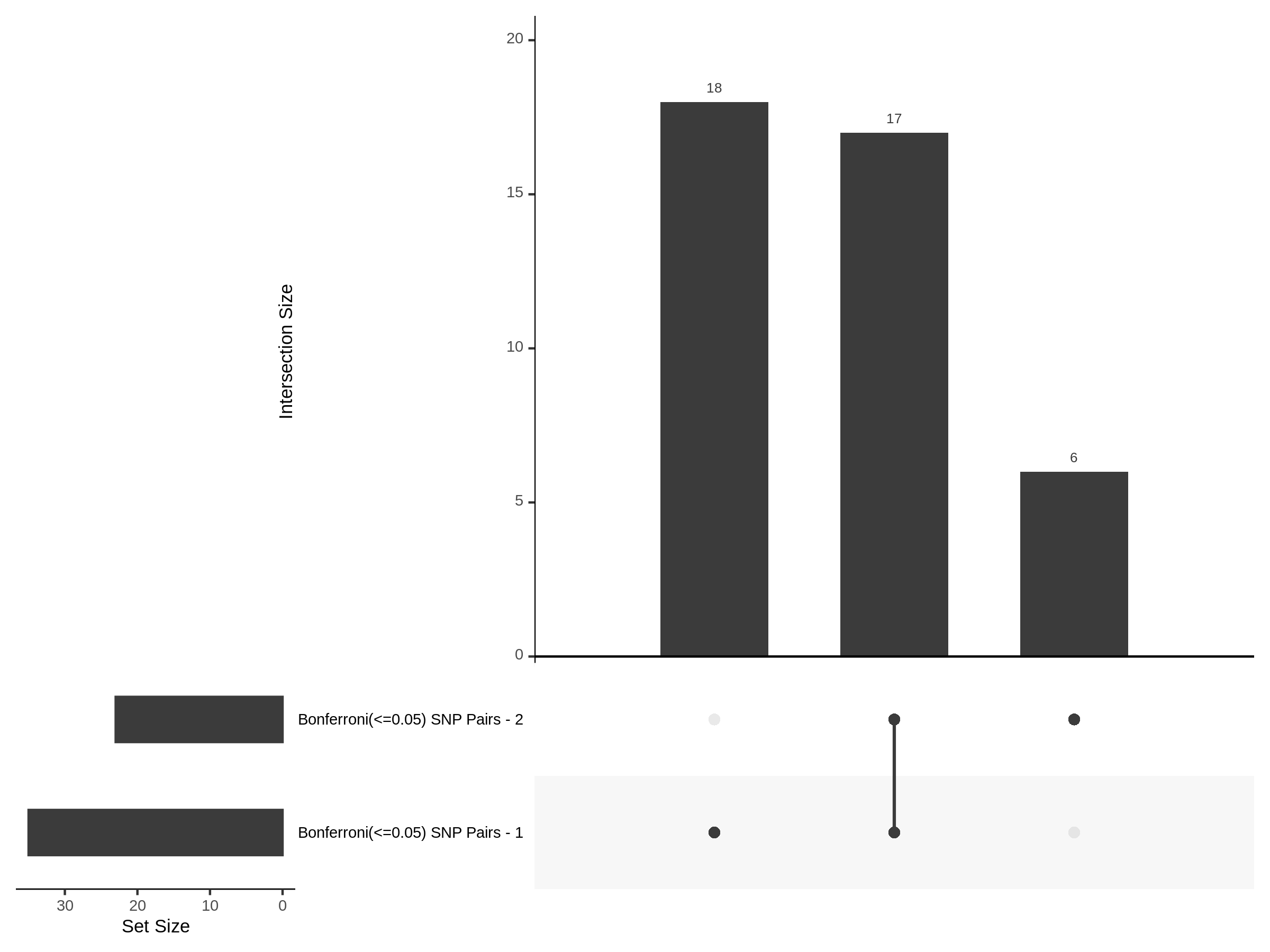
Scatterplot of PTC signals:
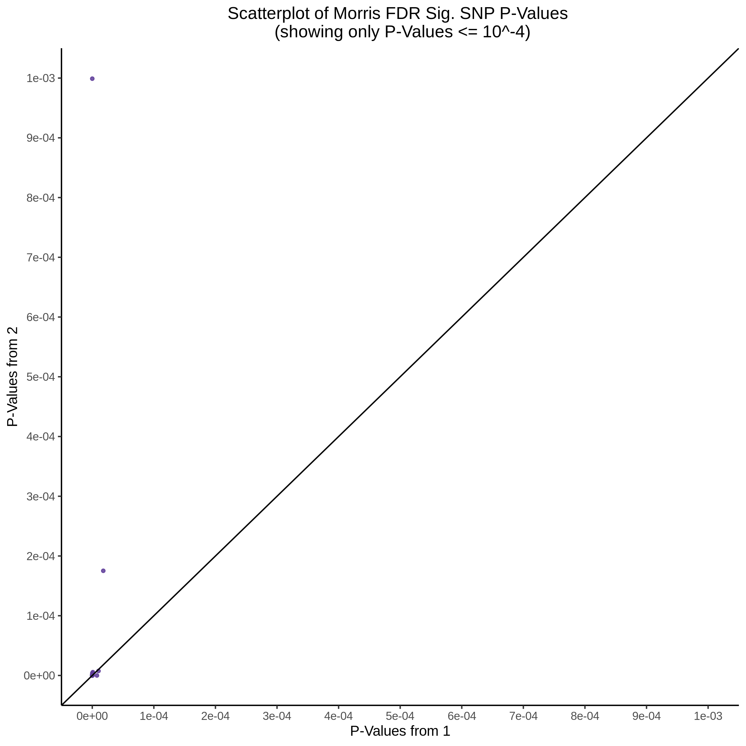
8/4/2022 gRNA matrix comparison: Morris dataset
Here we plot each gRNA (210 total: SNP, PTC, NTC subtypes) as a point, and we define the axiis as the proportion of cells (out of 9343 cells reported in supplment) that contain a gRNA after a 5 UMI threshold is applied. Cells with UMI counts lower than the threshold are considered zeroes/dont contain a gRNA. This is done to simulate the threshold later used to binarize the gRNA matrix during SCEPTRE.
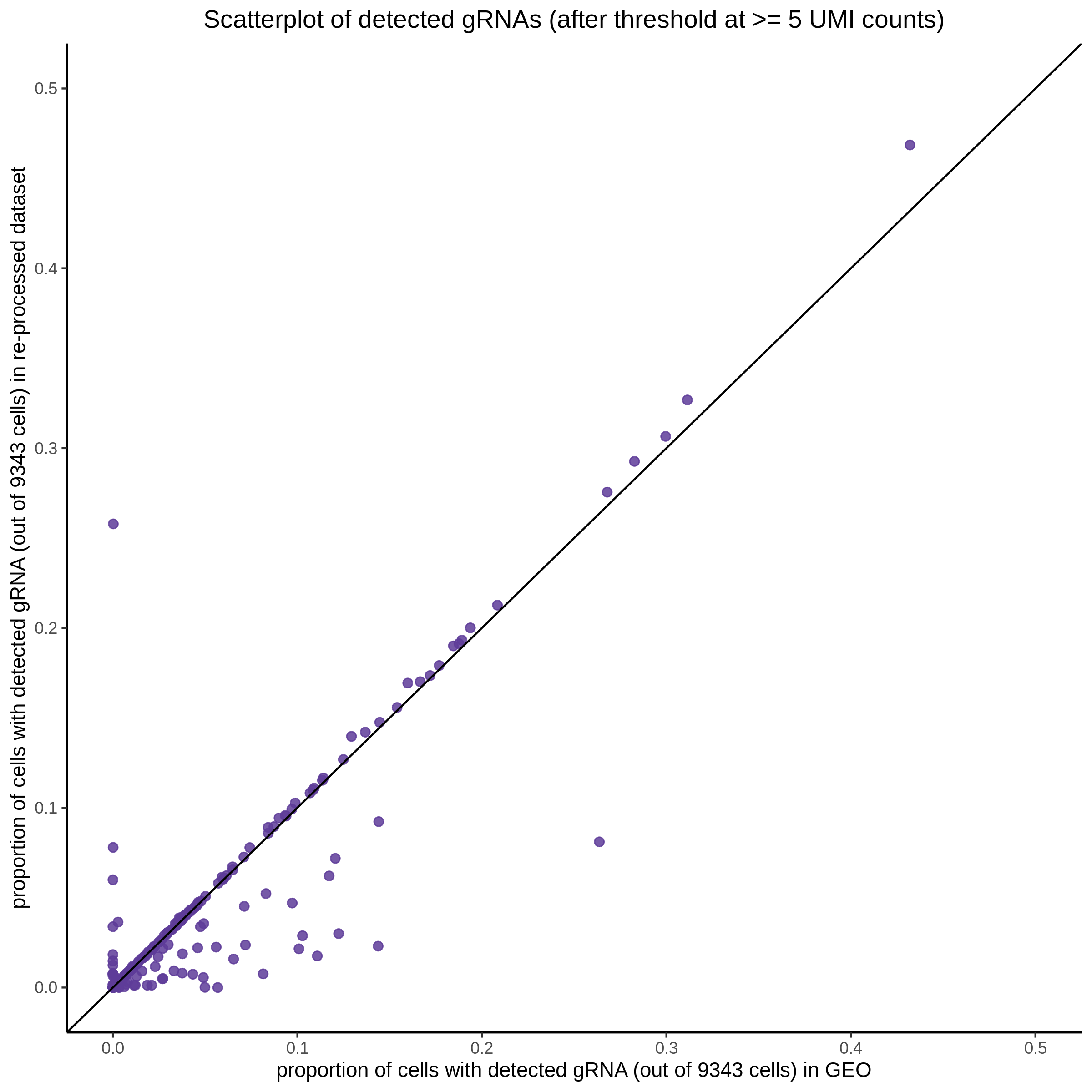
Here we plot the same set of gRNAs (210) across the same set of cells (9343) as above but we change our definition of detectability to be simply non zero UMI counts (>= 1 UMI). For example, a gRNA is ‘detected’ if a cell has at least 1 UMI corresponding to that gRNA.
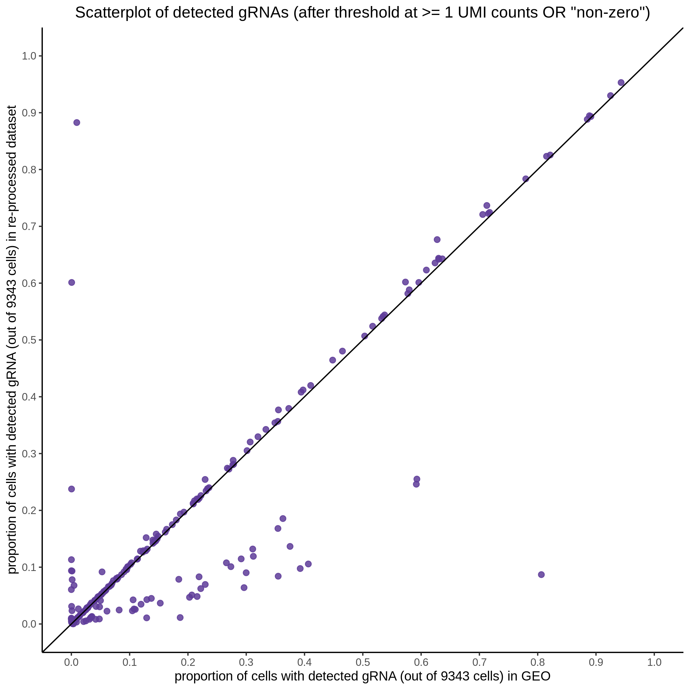
Below is a table of each of the proportions per gRNA based on the >= 5 UMI threshold (plot #1 above).
| gRNAs | geo_matrix_gRNAs | reprocessed_matrix_gRNAs |
|---|---|---|
| SNP-11_1 | 0.0322166 | 0.0324307 |
| SNP-11_2 | 0.0072782 | 0.0072782 |
| SNP-1_1 | 0.0089907 | 0.0090977 |
| SNP-26_2 | 0.1140961 | 0.1164508 |
| SNP-26_1 | 0.0225838 | 0.0226908 |
| SNP-1_2 | 0.0138071 | 0.0143423 |
| SNP-28_1 | 0.1249063 | 0.1268329 |
| SNP-28_2 | 0.0396018 | 0.0401370 |
| SNP-20_1 | 0.0068500 | 0.0071711 |
| SNP-20_2 | 0.1597988 | 0.1693246 |
| SNP-82_1 | 0.0370331 | 0.0389596 |
| SNP-13_2 | 0.0364979 | 0.0369260 |
| SNP-13_1 | 0.0421706 | 0.0432409 |
| SNP-82_2 | 0.0649684 | 0.0655036 |
| SNP-55_2 | 0.0176603 | 0.0176603 |
| SNP-80_2 | 0.1107781 | 0.0175532 |
| SNP-80_1 | 0.0711763 | 0.0451675 |
| SNP-75_2 | 0.0653966 | 0.0158407 |
| SNP-75_1 | 0.0001070 | 0.0001070 |
| SNP-22_2 | 0.0313604 | 0.0317885 |
| SNP-22_1 | 0.0111313 | 0.0113454 |
| SNP-86_1 | 0.0338221 | 0.0356417 |
| SNP-74_2 | 0.0248314 | 0.0252596 |
| SNP-86_2 | 0.2995826 | 0.3065397 |
| SNP-49_2 | 0.0024617 | 0.0029969 |
| SNP-58_1 | 0.0080274 | 0.0081344 |
| SNP-58_2 | 0.0460238 | 0.0463449 |
| SNP-49_1 | 0.0416354 | 0.0420636 |
| SNP-7_2 | 0.0474152 | 0.0338221 |
| SNP-7_1 | 0.0050305 | 0.0034250 |
| SNP-36_1 | 0.0433480 | 0.0073852 |
| SNP-36_2 | 0.0000000 | 0.0001070 |
| SNP-53_2 | 0.0971851 | 0.0469870 |
| SNP-53_1 | 0.0568340 | 0.0000000 |
| SNP-74_1 | 0.1135610 | 0.1152735 |
| SNP-34_2 | 0.1540191 | 0.1557316 |
| SNP-34_1 | 0.0439902 | 0.0443112 |
| SNP-5_1 | 0.0033180 | 0.0038532 |
| SNP-5_2 | 0.0741732 | 0.0778123 |
| SNP-55_1 | 0.0601520 | 0.0610082 |
| SNP-24_2 | 0.0600450 | 0.0605801 |
| SNP-85_2 | 0.0021406 | 0.0021406 |
| SNP-85_1 | 0.1891255 | 0.1931928 |
| HSPA8-2 | 0.1223376 | 0.0299690 |
| SNP-32_1 | 0.0120946 | 0.0012844 |
| SNP-32_2 | 0.0000000 | 0.0001070 |
| HSPA8-1 | 0.1440651 | 0.0922616 |
| SNP-15_1 | 0.0021406 | 0.0022477 |
| SNP-3_2 | 0.0378893 | 0.0381034 |
| SNP-3_1 | 0.1768169 | 0.1790645 |
| SNP-15_2 | 0.0452745 | 0.0453816 |
| SNP-51_1 | 0.0000000 | 0.0147704 |
| CD55-8 | 0.0009633 | 0.0005352 |
| SNP-17_2 | 0.0376753 | 0.0187306 |
| SNP-17_1 | 0.0459167 | 0.0220486 |
| CD55-9 | 0.0101680 | 0.0103821 |
| SNP-41_2 | 0.0082415 | 0.0085626 |
| SNP-57_2 | 0.0002141 | 0.0003211 |
| SNP-57_1 | 0.0492347 | 0.0355346 |
| SNP-41_1 | 0.0064219 | 0.0067430 |
| SNP-51_2 | 0.0000000 | 0.0016055 |
| SNP-30_2 | 0.0184095 | 0.0186236 |
| SNP-30_1 | 0.0132720 | 0.0132720 |
| SNP-73_2 | 0.0295408 | 0.0305041 |
| SNP-25_1 | 0.0000000 | 0.0599379 |
| SNP-25_2 | 0.0000000 | 0.0066360 |
| SNP-19_1 | 0.0253666 | 0.0254736 |
| SNP-8_1 | 0.0409933 | 0.0420636 |
| SNP-8_2 | 0.1845232 | 0.1899818 |
| SNP-19_2 | 0.0019266 | 0.0019266 |
| RPL22-2 | 0.0351065 | 0.0366049 |
| RPL22-1 | 0.0369260 | 0.0374612 |
| SNP-27_2 | 0.0187306 | 0.0187306 |
| SNP-27_1 | 0.1090656 | 0.1108852 |
| CD55-3 | 0.0000000 | 0.0000000 |
| SNP-65_1 | 0.0004281 | 0.0003211 |
| SNP-65_2 | 0.0002141 | 0.0000000 |
| CD55-10 | 0.0000000 | 0.0014984 |
| SNP-21_1 | 0.0216205 | 0.0217275 |
| SNP-21_2 | 0.1367869 | 0.1420315 |
| SNP-12_2 | 0.0969710 | 0.0992187 |
| SNP-83_1 | 0.0032110 | 0.0002141 |
| SNP-83_2 | 0.0814514 | 0.0075993 |
| SNP-12_1 | 0.0099540 | 0.0100610 |
| NTC-12 | 0.0933319 | 0.0956866 |
| SNP-81_2 | 0.0718185 | 0.0236541 |
| SNP-81_1 | 0.0001070 | 0.0000000 |
| SNP-38_2 | 0.0614364 | 0.0621856 |
| NTC-11 | 0.0070641 | 0.0070641 |
| SNP-38_1 | 0.1068179 | 0.1082094 |
| NTC-10 | 0.0369260 | 0.0374612 |
| SNP-23_2 | 0.0000000 | 0.0000000 |
| SNP-23_1 | 0.0268650 | 0.0048164 |
| SNP-71_2 | 0.0014984 | 0.0014984 |
| SNP-71_1 | 0.0212994 | 0.0215134 |
| SNP-6_2 | 0.0459167 | 0.0467730 |
| SNP-35_2 | 0.0157337 | 0.0161618 |
| SNP-35_1 | 0.0648614 | 0.0671091 |
| SNP-6_1 | 0.0345713 | 0.0347854 |
| SNP-77_1 | 0.0085626 | 0.0086696 |
| SNP-77_2 | 0.0369260 | 0.0372471 |
| SNP-33_1 | 0.0221556 | 0.0222627 |
| SNP-33_2 | 0.0058868 | 0.0058868 |
| SNP-4_1 | 0.0559777 | 0.0224767 |
| SNP-4_2 | 0.0209783 | 0.0012844 |
| SNP-24_1 | 0.0069571 | 0.0070641 |
| SNP-2_2 | 0.1718934 | 0.1734989 |
| SNP-14_1 | 0.0174462 | 0.0174462 |
| SNP-14_2 | 0.0590817 | 0.0613293 |
| SNP-2_1 | 0.0366049 | 0.0384245 |
| SNP-31_2 | 0.0001070 | 0.0002141 |
| SNP-31_1 | 0.0011774 | 0.0011774 |
| SNP-16_2 | 0.0490207 | 0.0055657 |
| SNP-16_1 | 0.0000000 | 0.0124157 |
| SNP-61_1 | 0.1446002 | 0.1474901 |
| SNP-61_2 | 0.0477363 | 0.0480574 |
| SNP-9_1 | 0.0031039 | 0.0032110 |
| SNP-62_2 | 0.0061008 | 0.0003211 |
| SNP-62_1 | 0.0033180 | 0.0000000 |
| SNP-9_2 | 0.0387456 | 0.0400300 |
| SNP-45_2 | 0.1008241 | 0.0215134 |
| SNP-45_1 | 0.0245103 | 0.0171251 |
| SNP-64_1 | 0.0168040 | 0.0171251 |
| SNP-18_1 | 0.0428128 | 0.0433480 |
| SNP-18_2 | 0.0291127 | 0.0295408 |
| SNP-64_2 | 0.0447394 | 0.0449534 |
| CD52-1 | 0.0105962 | 0.0117735 |
| NTC-9 | 0.0598309 | 0.0602590 |
| CD52-2 | 0.1172000 | 0.0620786 |
| CD55-2 | 0.0000000 | 0.0077063 |
| SNP-43_1 | 0.0000000 | 0.0338221 |
| SNP-43_2 | 0.0000000 | 0.0078133 |
| CD55-1 | 0.0462378 | 0.0474152 |
| CD55-6 | 0.0000000 | 0.0183025 |
| CD55-7 | 0.1205180 | 0.0718185 |
| CD55-4 | 0.2636198 | 0.0810232 |
| CD55-5 | 0.0000000 | 0.0002141 |
| NTC-7 | 0.0009633 | 0.0010703 |
| NTC-6 | 0.0842342 | 0.0858397 |
| NTC-5 | 0.0709622 | 0.0725677 |
| NTC-4 | 0.0296479 | 0.0306112 |
| NTC-3 | 0.2083913 | 0.2126726 |
| NTC-2 | 0.1292947 | 0.1396768 |
| NTC-1 | 0.0072782 | 0.0078133 |
| SNP-39_2 | 0.0111313 | 0.0113454 |
| SNP-39_1 | 0.2826715 | 0.2926255 |
| NTC-8 | 0.2679011 | 0.2755004 |
| SNP-63_2 | 0.0987905 | 0.1026437 |
| SNP-73_1 | 0.0872311 | 0.0894788 |
| SNP-10_1 | 0.0000000 | 0.0000000 |
| CD46-2 | 0.0375682 | 0.0080274 |
| SNP-37_1 | 0.0162689 | 0.0163759 |
| SNP-10_2 | 0.0270791 | 0.0217275 |
| PPIA-1 | 0.0048164 | 0.0049235 |
| SNP-37_2 | 0.0220486 | 0.0223697 |
| SNP-63_1 | 0.0938671 | 0.0953655 |
| NMU-2 | 0.3113561 | 0.3267687 |
| SNP-70_2 | 0.0186236 | 0.0012844 |
| SNP-70_1 | 0.0000000 | 0.0074922 |
| SNP-78_2 | 0.1085305 | 0.1099219 |
| SNP-78_1 | 0.0168040 | 0.0169111 |
| SNP-76_1 | 0.0359628 | 0.0387456 |
| SNP-76_2 | 0.0900139 | 0.0942952 |
| SNP-66_2 | 0.0017125 | 0.0054586 |
| SNP-66_1 | 0.0001070 | 0.0779193 |
| PPIA-2 | 0.4319812 | 0.4685861 |
| SNP-60_1 | 0.1437440 | 0.0230119 |
| SNP-60_2 | 0.0498769 | 0.0001070 |
| SNP-68_1 | 0.0265439 | 0.0268650 |
| SNP-47_1 | 0.0571551 | 0.0580113 |
| SNP-47_2 | 0.0064219 | 0.0064219 |
| SNP-68_2 | 0.1665418 | 0.1700739 |
| SNP-44_2 | 0.0002141 | 0.2578401 |
| SNP-44_1 | 0.0027828 | 0.0363909 |
| SNP-69_1 | 0.0204431 | 0.0205501 |
| SNP-69_2 | 0.0278283 | 0.0288986 |
| SNP-87_1 | 0.0396018 | 0.0406722 |
| SNP-87_2 | 0.0340362 | 0.0341432 |
| SNP-42_1 | 0.0002141 | 0.0000000 |
| SNP-42_2 | 0.0113454 | 0.0012844 |
| SNP-29_1 | 0.0363909 | 0.0366049 |
| SNP-29_2 | 0.1875201 | 0.1912662 |
| SNP-88_2 | 0.0057797 | 0.0057797 |
| SNP-88_1 | 0.0012844 | 0.0012844 |
| SNP-59_1 | 0.0501980 | 0.0507332 |
| SNP-48_2 | 0.0222627 | 0.0229048 |
| SNP-48_1 | 0.0841272 | 0.0890506 |
| SNP-59_2 | 0.0222627 | 0.0222627 |
| SNP-67_2 | 0.1027507 | 0.0287916 |
| SNP-72_1 | 0.0299690 | 0.0238681 |
| SNP-72_2 | 0.0229048 | 0.0116665 |
| SNP-50_1 | 0.0357487 | 0.0364979 |
| SNP-50_2 | 0.0400300 | 0.0408862 |
| SNP-79_2 | 0.0094188 | 0.0099540 |
| SNP-79_1 | 0.1937279 | 0.2000428 |
| SNP-67_1 | 0.0829498 | 0.0522316 |
| SNP-52_2 | 0.0191587 | 0.0198009 |
| SNP-52_1 | 0.0092048 | 0.0094188 |
| SNP-84_2 | 0.0000000 | 0.0000000 |
| SNP-84_1 | 0.0001070 | 0.0000000 |
| CD46-1 | 0.0004281 | 0.0001070 |
| SNP-54_1 | 0.0270791 | 0.0050305 |
| SNP-54_2 | 0.0000000 | 0.0002141 |
| SNP-40_2 | 0.0070641 | 0.0018195 |
| SNP-40_1 | 0.0002141 | 0.0004281 |
| NMU-1 | 0.0062079 | 0.0066360 |
| SNP-46_1 | 0.0330729 | 0.0093118 |
| SNP-46_2 | 0.0157337 | 0.0090977 |
| SNP-56_2 | 0.0127368 | 0.0063149 |
| SNP-56_1 | 0.0079204 | 0.0031039 |
SNP 44-2
From these scatter plots we see that several gRNAs are starkly different between datasets. While most gRNAs are found in an equal proportion of the same 9343 cells, some do not fall on the 1:1 line (black line above).
For example: SNP 44-2 appears to be barely detected (~ 0 proportion => ~ 0 cells) while in the reprocessed gRNA matrix that same gRNA was detected with a threshold >= 5 UMIs in almost ~0.25 or 25% of cells (9343 cells => ~ 2225 cells). This is strange because we are comparing the same group of cells (9343 cell barcodes) so the cells should have roughly the same gRNA “content” by raw UMI counts and by detectability (thresholded UMI counts).
Taking a closer look at particularly which cells had SNP-44-2 and what exactly are the UMI counts:
# First we are going to inspect the GEO gRNA matrix:
# load original paper matrix
GDO = '/project/xuanyao/nikita/SCEPTRE/data/Morris_2021/GSM5225858_GDO.mtx.gz'
GDO_cbc = '/project/xuanyao/nikita/SCEPTRE/data/Morris_2021/GSM5225858_GDO.barcodes.txt'
GDO_features = '/project/xuanyao/nikita/SCEPTRE/data/Morris_2021/GSM5225858_GDO.features.txt'
f_grna_matrix = ReadMtx(mtx = GDO, features = GDO_features, cells = GDO_cbc, cell.column=1, feature.column=1, mtx.transpose=T)

# pull out those >= 5 UMI counts in GEO
THRESHOLD_cells =  (f_grna_matrix['SNP-44_2', paper_cbcs])[ (f_grna_matrix['SNP-44_2', paper_cbcs]) >= 5] # 2 total

# pull out those >= 1 UMI counts in GEO
non_zero_cells =  (f_grna_matrix['SNP-44_2', paper_cbcs])[ (f_grna_matrix['SNP-44_2', paper_cbcs]) >= 1] # 87 total
Here are the cell-level UMI counts for SNP 44-2 in the GEO gRNA dataset:
r$> THRESHOLD_cells  # showing 2 / 2
CAGATCAGTTCAGGCC TCATTACGTAACGACG
               5               11

r$> non_zero_cells # showing 31 / 87
              umis         barcodes
 1:              1 AACCGCGGTACAGTTC
 2:              4 AACCGCGTCAGTCAGT
 3:              1 AAGCCGCGTTTGTGTG
 4:              1 AAGTCTGAGGACGAAA
 5:              1 AATCCAGCATTCTCAT
 6:              1 ACACCCTCAAAGTCAA
 7:              1 ACATCAGTCGAGAACG
 8:              1 ACCCACTCATGCCTAA
 9:              1 ACCCACTGTTATCCGA
10:              1 ACCCACTGTTGCGTTA
11:              1 ACGAGCCAGAAACCTA
12:              1 ACGCAGCCAGGACGTA
13:              1 ACGGAGACATCAGTAC
14:              1 ACGGCCACACAACGTT
15:              1 ACTTGTTGTATTACCG
16:              1 AGAATAGCACAGTCGC
17:              1 AGGGTGAAGTCTCCTC
18:              1 AGTGTCAAGTTACCCA
19:              1 ATCATCTAGCCAGGAT
20:              1 ATCCGAAGTCCGCTGA
21:              1 ATGAGGGAGCGTGTCC
22:              1 ATGGGAGCACGGATAG
23:              1 ATTACTCAGTTAACGA
24:              1 CACACCTCAATGTAAG
25:              1 CACCTTGTCGGCGCAT
26:              1 CACTCCATCCCTCAGT
27:              1 CAGAATCTCATTTGGG
28:              1 CAGAATCTCTGGCGAC
29:              5 CAGATCAGTTCAGGCC
30:              1 CAGCTGGAGCACCGTC
31:              1 CAGTAACGTCTTCGTC
Now we look to the reprocessed gRNA dataset, showing just the results from THRESHOLD_cells (>= 5 UMIs) we see a completely different story for this gRNA.
THRESHOLD_cells = (gRNA_matrix['SNP-44_2', paper_cbcs])[ (gRNA_matrix['SNP-44_2', paper_cbcs]) >= 5] # (2409 total) kallisto-bustools reprocessed gRNA matrix

r$> THRESHOLD_cells[1:40,] # first 40 cells / 2409
    umis         barcodes
 1:    8 AAACCTGAGCCCAGCT
 2:    7 AAACCTGCATGCAACT
 3:    5 AAACCTGGTCATATCG
 4:    5 AAACCTGTCAAAGTAG
 5:    5 AAACGGGAGACCACGA
 6:   22 AAACGGGCAATCTACG
 7:    6 AAACGGGCACATGTGT
 8:   73 AAACGGGCACATTCGA
 9:    9 AAACGGGGTAAACCTC
10:    7 AAACGGGGTCGGATCC
11:  290 AAACGGGTCGCACTCT
12:    5 AAAGATGAGAGGTAGA
13:    5 AAAGATGAGCGATATA
14:  109 AAAGATGCAGCTCGCA
15:    5 AAAGATGCATAAAGGT
16:    5 AAAGATGGTCTGCGGT
17:   20 AAAGATGTCGTATCAG
18:    5 AAAGATGTCGTTACGA
19:    7 AAAGCAAAGAGTGAGA
20:    5 AAAGCAACAGCGTCCA
21:  204 AAAGCAACAGGACCCT
22:    9 AAAGCAAGTTACTGAC
23:   31 AAAGCAATCACTTCAT
24:    5 AAAGCAATCAGCAACT
25:    5 AAAGCAATCTTCTGGC
26:    8 AAAGTAGAGGCATGGT
27:  309 AAAGTAGCACATGACT
28:  134 AAAGTAGCAGTGGGAT
29:   93 AAAGTAGGTCTGCAAT
30:    7 AAAGTAGGTGTGGCTC
31:  172 AAAGTAGTCCAGATCA
32:  344 AAATGCCAGATGCGAC
33:  469 AAATGCCAGTATCGAA
34:    7 AAATGCCCAAGTAGTA
35:  319 AAATGCCCACACCGAC
36:    5 AAATGCCCAGATAATG
37:    9 AAATGCCGTCCTAGCG
38:    6 AACACGTCATCGGACC
39:    6 AACACGTGTCGCATCG
40:  107 AACACGTGTGAGGGAG
From this we see that most GEO UMI counts for SNP-44-2 are close to zero, with 85 (/87 cells nonzero) cells containing between 1-4 UMIs. For the reprocessed dataset this is the opposite: most UMI counts for SNP 44-2 are >= 5, with 2409/9343 cells containing >=5 UMIs.
Plotting the histograms of all non zero cells for SNP 44-2:
GEO
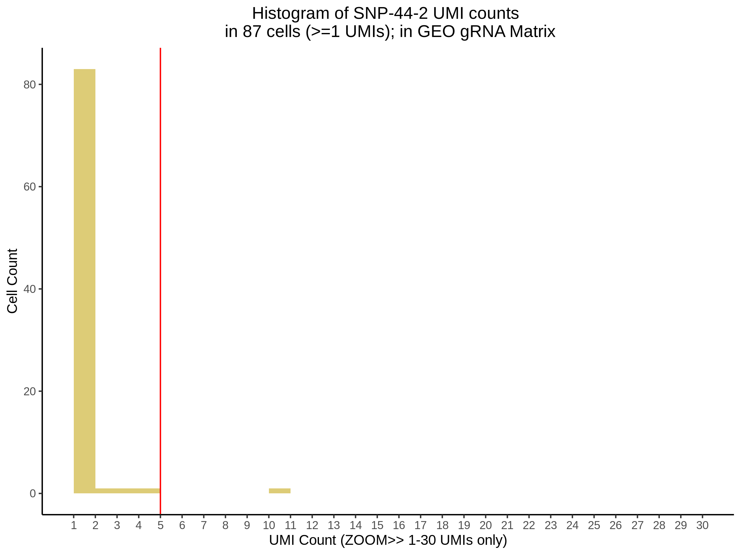
Re-Processed
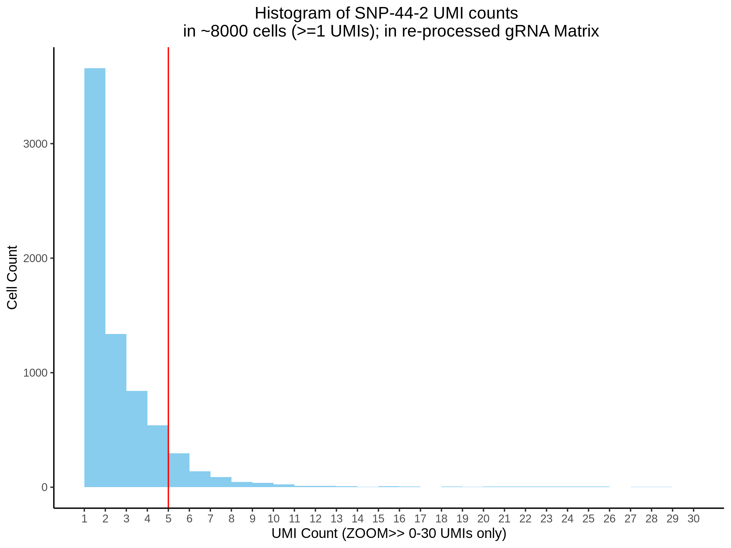
8/3/2022 QQPlots and PValue Histograms Associated with GEO/re-processed Morris Data
Here we plot the QQplots and p value histrograms associated with the SCEPTRE results from GEO vs those from the re-processed dataset. We specifically investigate the NTC qqplots and histograms in order to look at the behaviour/detectability of problem NTCs which refers to when NTCs produce a phenotype signal by chance (Replogle et al. Cell. 2022)
Morris GEO
All NTCs QQplot + Histogram
![]()
![]()
![]()
![]()
![]()
![]()
![]()
![]()
![]()
![]()
![]()
![]()
![]()
![]()
NTC pairs removing NTC-3, 8, and 11.
![]()
![]()
PTC QQplot + Histogram
![]()
![]()
SNP QQplot + Histogram
![]()
![]()
Morris re-processed
Here we do the same but for the re-processed dataset (raw data > UMI count matrixes > QC > SCEPTRE).
All NTCs QQplot + Histogram
![]()
![]()
![]()
![]()
![]()
![]()
![]()
![]()
![]()
![]()
![]()
![]()
![]()
![]()
NTC pairs removing NTC-3, 8, and 11.
![]()
![]()
PTC QQplot + Histogram
![]()
![]()
SNP QQplot + Histogram
![]()
![]()
Morris re-processed and adjusted for mappability
Here we do the same but for the re-processed dataset that used a mappability adjusted GTF reference (raw data > UMI count matrixes > QC > SCEPTRE).
All NTCs QQplot + Histogram
![]()
![]()
![]()
![]()
![]()
![]()
![]()
![]()
![]()
![]()
![]()
![]()
![]()
![]()
NTC pairs removing NTC-3, 8, and 11.
![]()
![]()
PTC QQplot + Histogram
![]()
![]()
SNP QQplot + Histogram
![]()
![]()
7/15/2022 Effect of Different Gene Definitions on Detectable Genes in Morris et al. 2021
Here we apply 3 different definitions for genes detected in the Morris dataset from GEO (cDNA matrix) and the re-processed Morris dataset output from CellRanger (filtered, cDNA matrix). We define genes as being well expressed or detectably expressed, including them in our downstream SCEPTRE analysis, if a read is present in at least 0.525%, 2% and 5% of all cells, respective to their datasets (GEO cDNA or pre-processed, filtered cDNA normal/mappablity adjusted). The size of each dataset in genes by cell and the amount of genes detected is shown below.
| Dataset | Size (genes x cell) | 0.525% of cell pop. | 2% of cell pop. | 5% of cell pop. |
|---|---|---|---|---|
| GEO cDNA dataset | 35606 x 680k | 15329 | 12052 | 10325 |
| re-processed cDNA dataset (normal) | 36601 x 15391 | 14579 | 11968 | 10345 |
| re-processed cDNA dataset (mappability adjusted) | 35580 x 13902 | 13689 | 11152 | 9462 |
7/13/2022 Morris re-Processed Dataset QC
This dataset is the Morris raw data for the cDNA, gRNA, and HTO matrixes that was processed accordingly: the cDNA reads were processed with CellRanger 7.0.0, the gRNA and HTO matrixes were processed according to the Kallisto-Bustools kite workflow. In both cases matrixes are generated and passed onto pre-processing in order to apply QC and prepare the data for SCEPTRE analysis.
re-Processed Dataset QC: ALL cells (directly from CellRanger 7.0.0 ‘filtered’ output), before QC applied
Plot of distribution of cells per gene as a histogram. A red line is
placed at 5% of 15,391 cells (770) as the minumum amount of cells a gene
must be found in, in order for it to be kept in the analysis. This is
used to filter out genes that are not found in most of the dataset and
that gene is not used later in association testing. 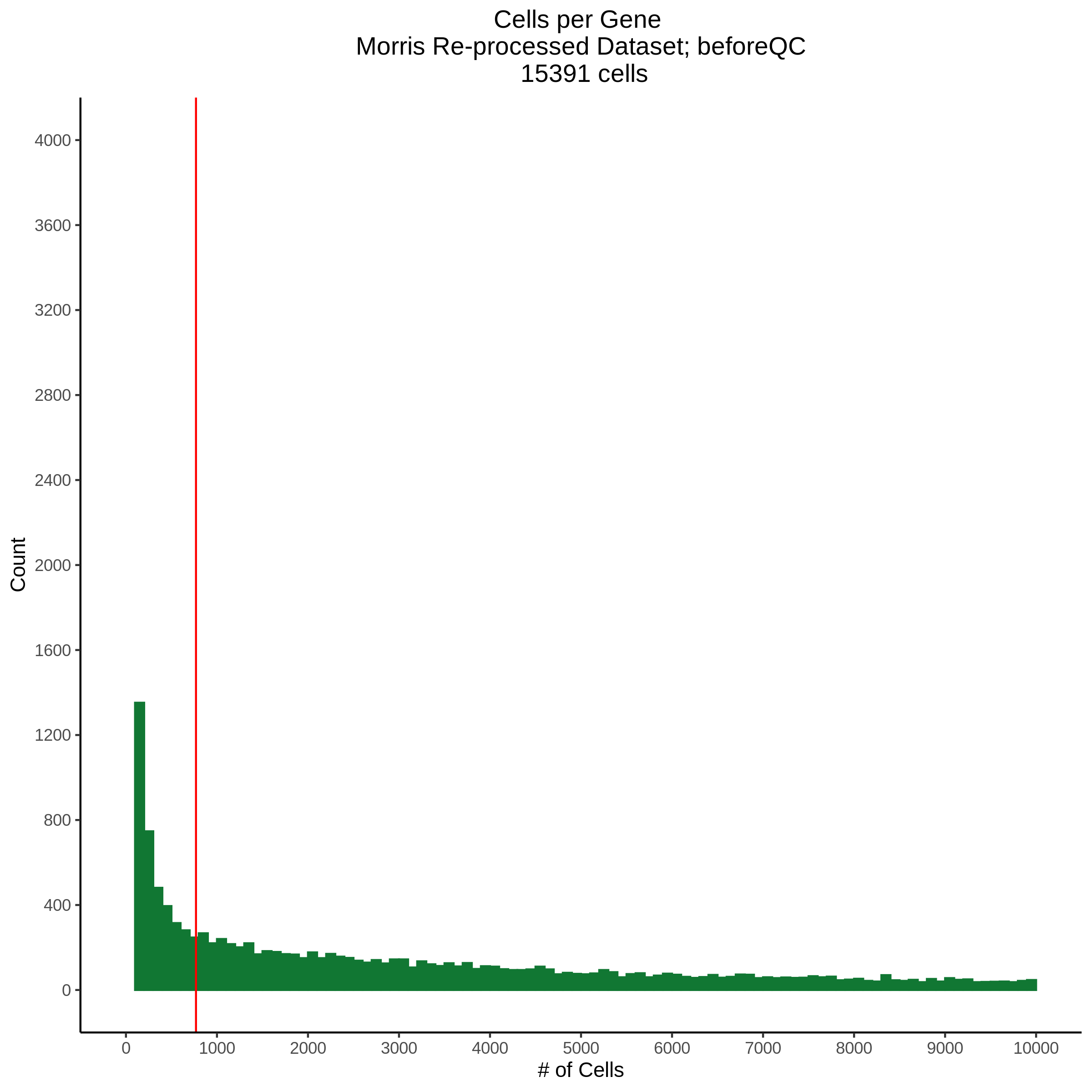
Plot of the distribution of genes per cell as a histogram. A red line
is placed at the current QC threshold of 850 unique genes. This
threshold does NOT appear to be appropriate for this dataset at the
moment. 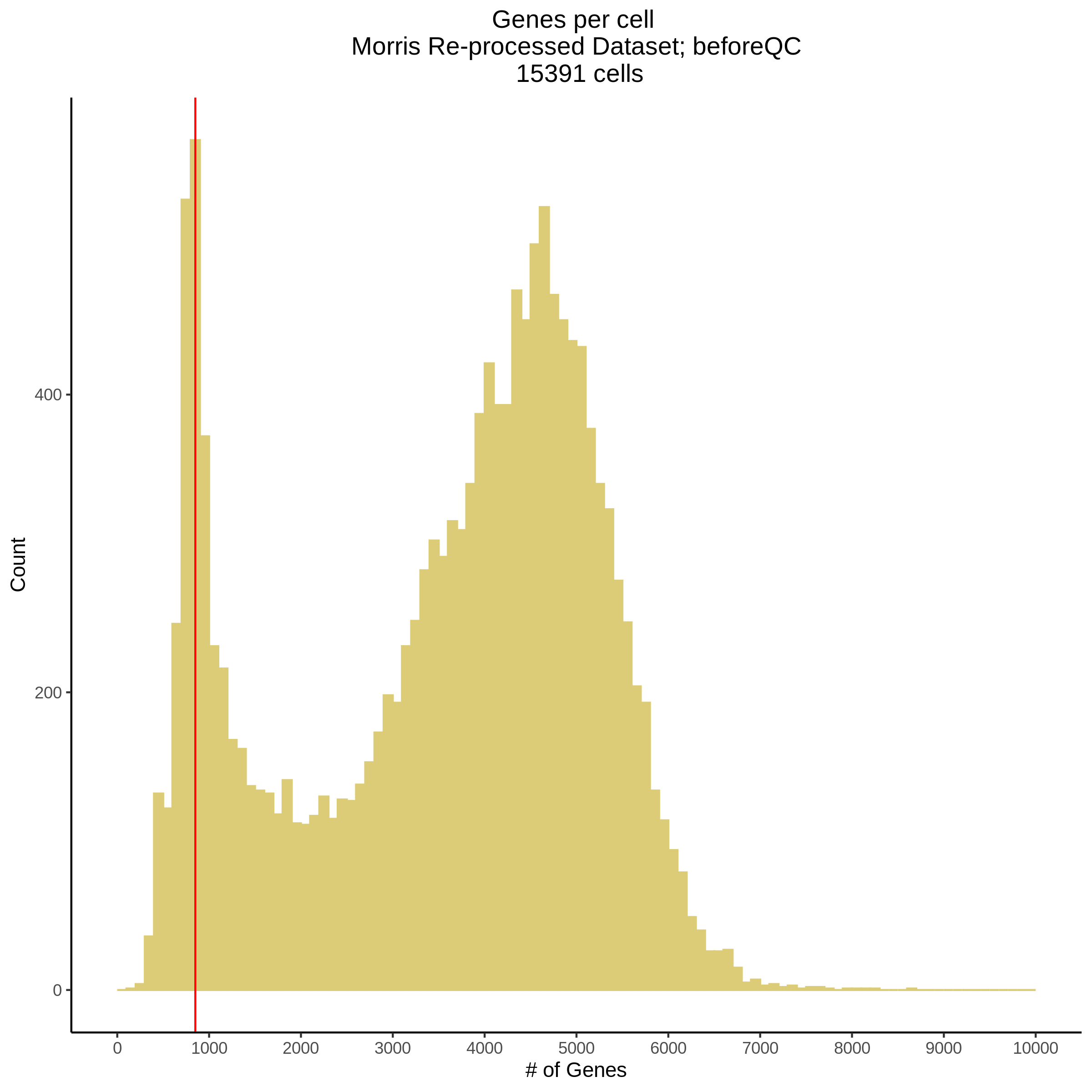
Plot of the count depth vs rank. The plot itself was introduced
originally in the Drop-seq paper (Macosko et al., Highly parallel
genome-wide expression profiling of individual cells using nanoliter
droplets, 2015.) Here you rank cells based on count depth to produce a
count depth (total UMIs) vs barcode rank plot and place a horizontal
threshold where the line curves down steeply. 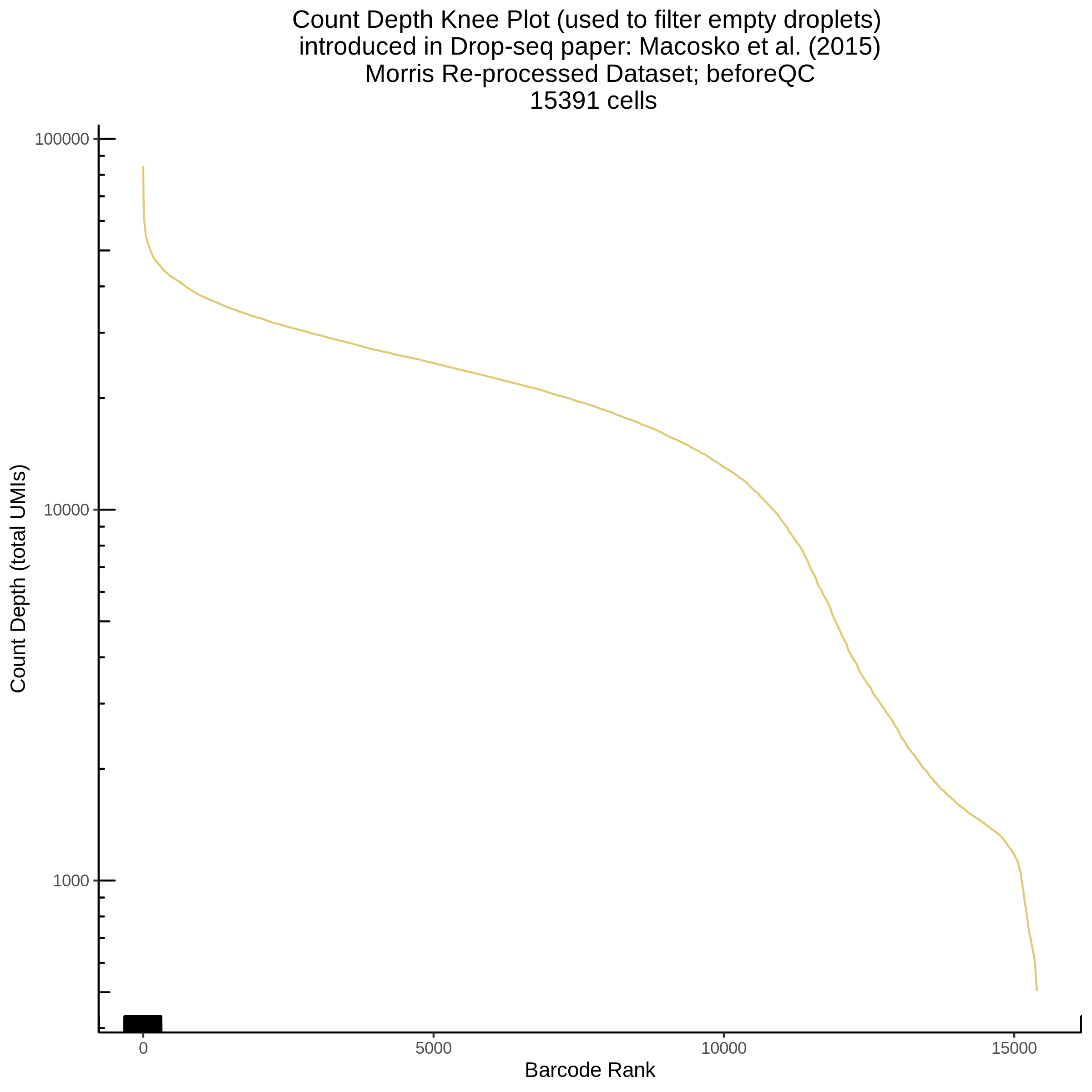
This is meant to be used in supplment to the plot above, where we
seek to define a lower bound for total UMI counts (count depth) based on
the distribution present in the data. 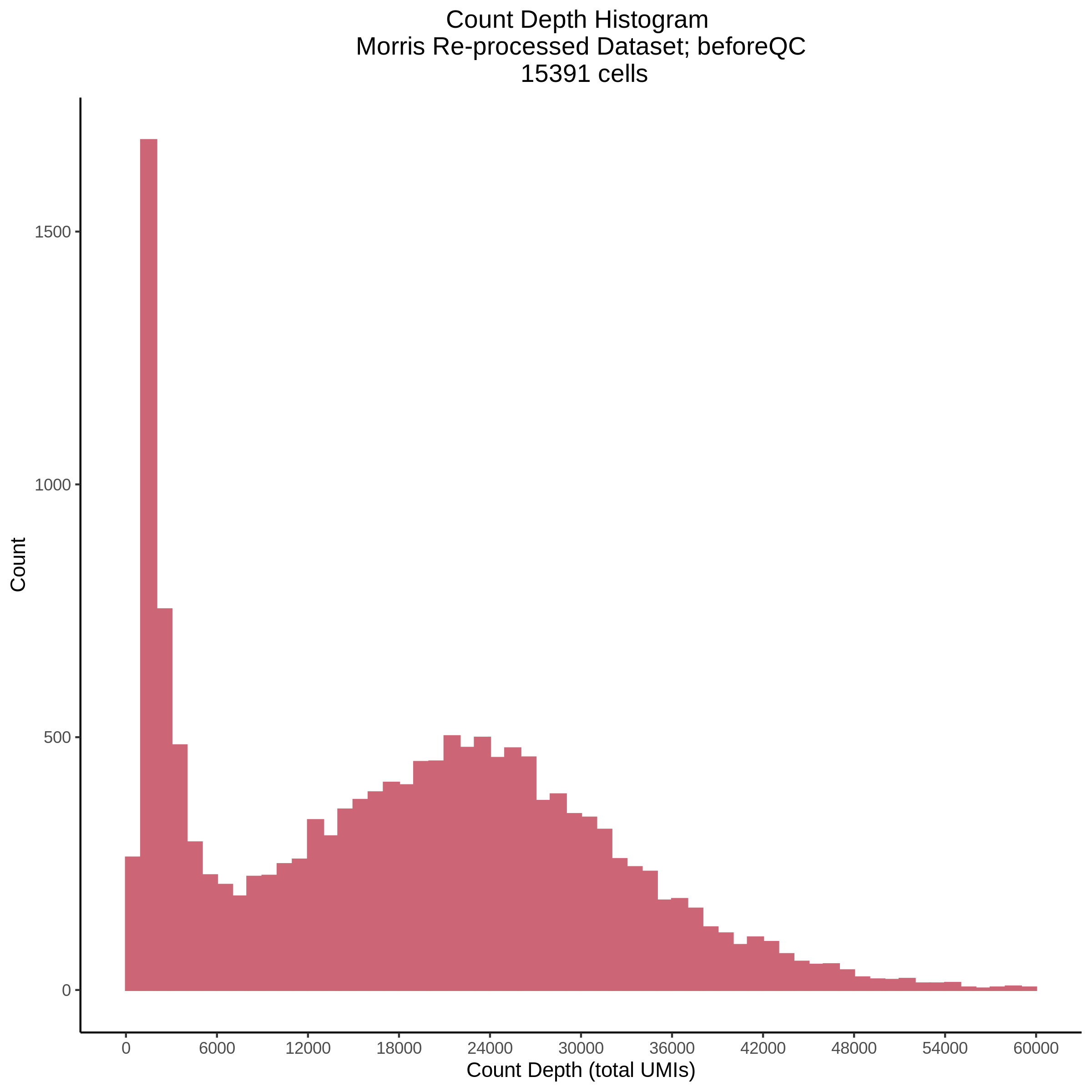
This plot is a scatter plot of count depth vs number of genes per
cell. This plot was taken from “Current best practices in scRNA-seq
analysis: a tutorial” Luecken & Theis. 2019 and to shows all cells
in the datasets as points. 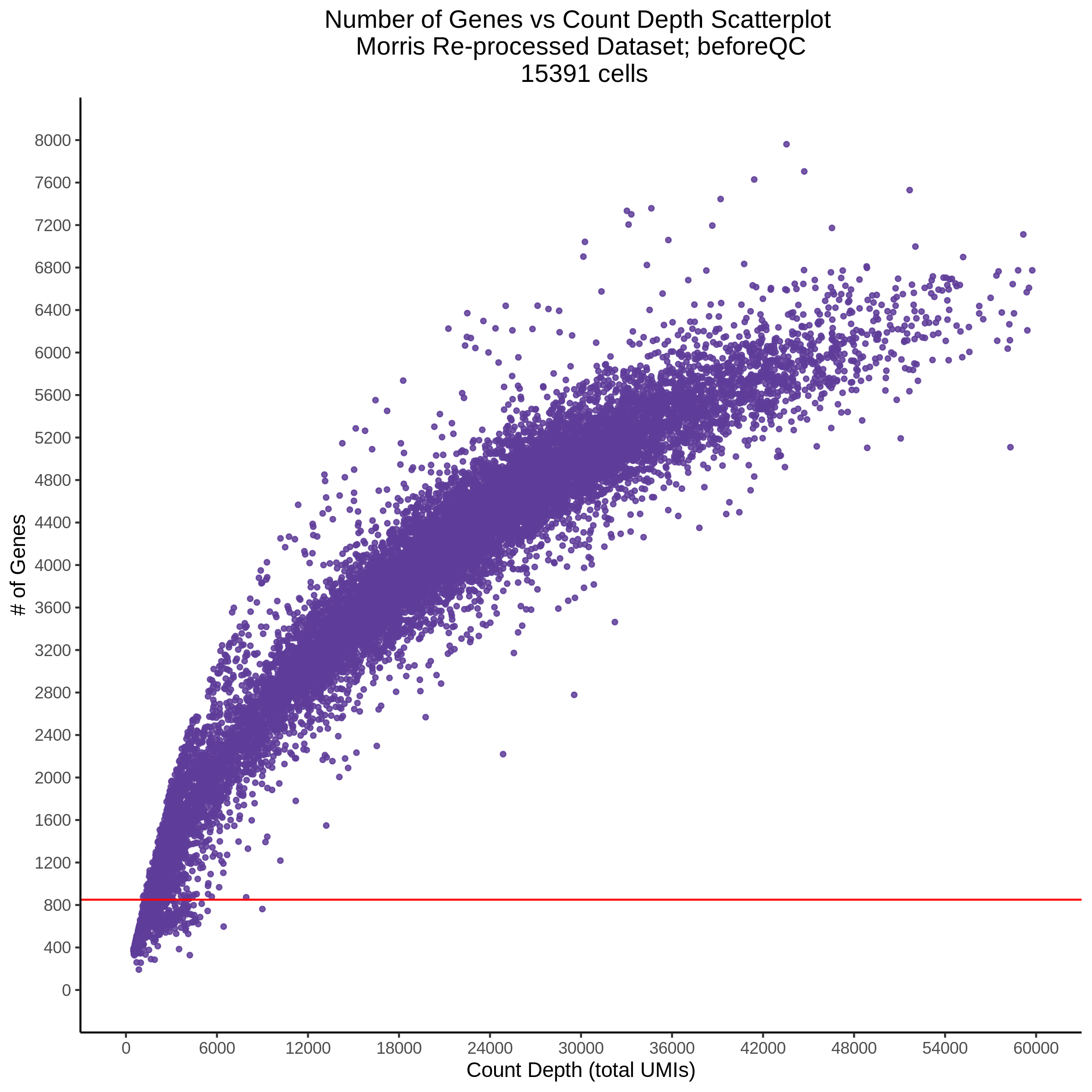
re-Processed Dataset QC: final SCEPTRE analysis cells, after QC applied
The following plots mirror those above but are made using the final, (input) expression and gRNA matrixes after QC. These plots serve to double check and visualize the final SCEPTRE ready dataset and shouldnt contain any concerns. Addional to the plots above, a MOI plot or gRNA per cell histogram is added to this section.
Plot of distribution of cells per gene as a histogram. A red line is
placed at 5% of the original 15,391 cells (770). 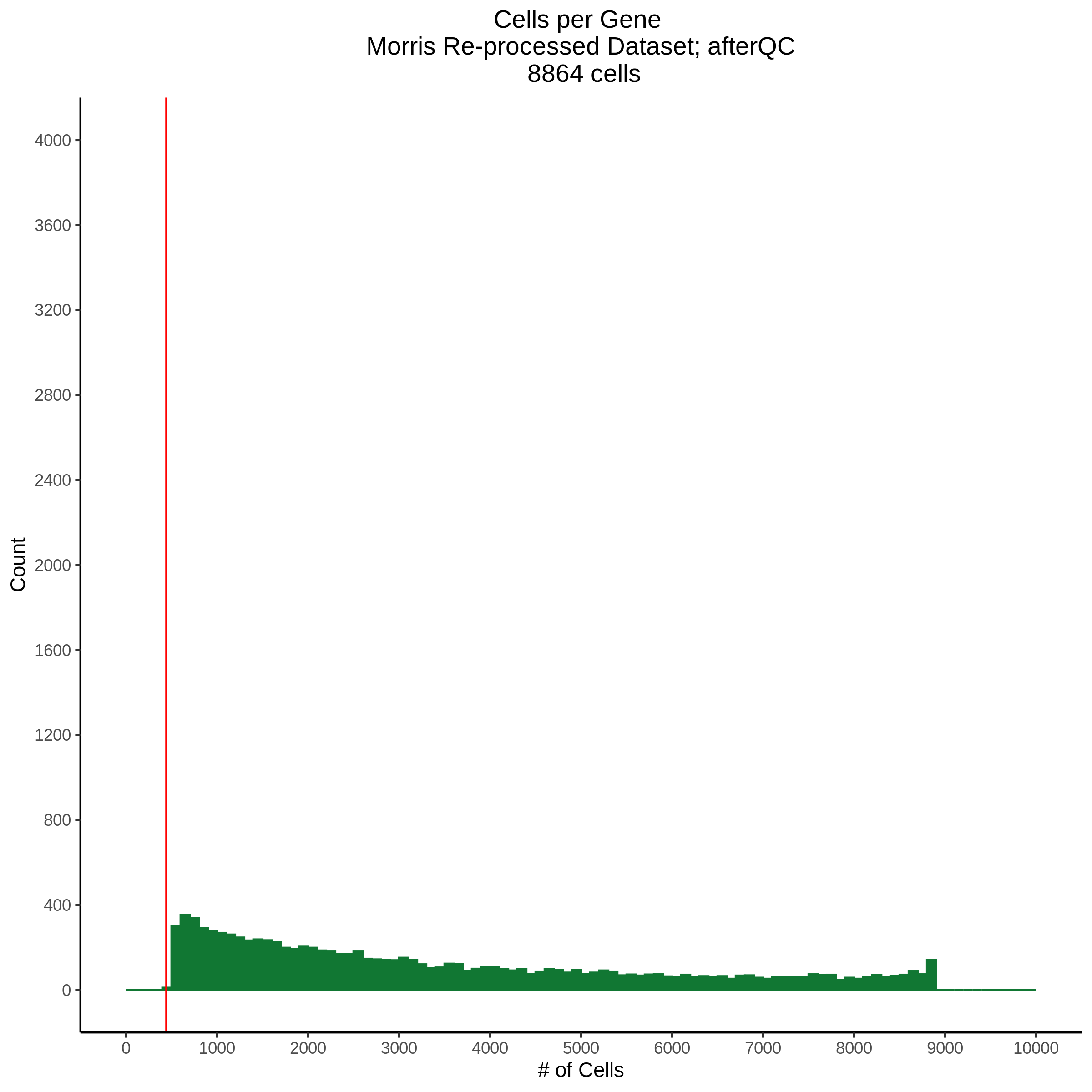
Plot of the distribution of genes per cell as a histogram. A red line
is placed at the current QC threshold of 850 unique genes. This
threshold does NOT appear to be appropriate for this dataset at the
moment. 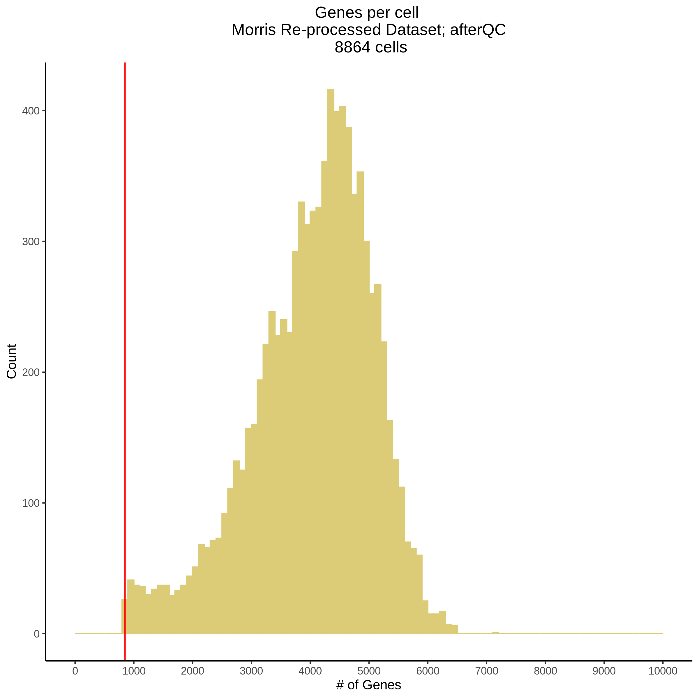
Plot of the count depth vs rank. The plot itself was introduced
originally in the Drop-seq paper (Macosko et al., Highly parallel
genome-wide expression profiling of individual cells using nanoliter
droplets, 2015.) Here you rank cells based on count depth to produce a
count depth (total UMIs) vs barcode rank plot and place a horizontal
threshold where the line curves down steeply. 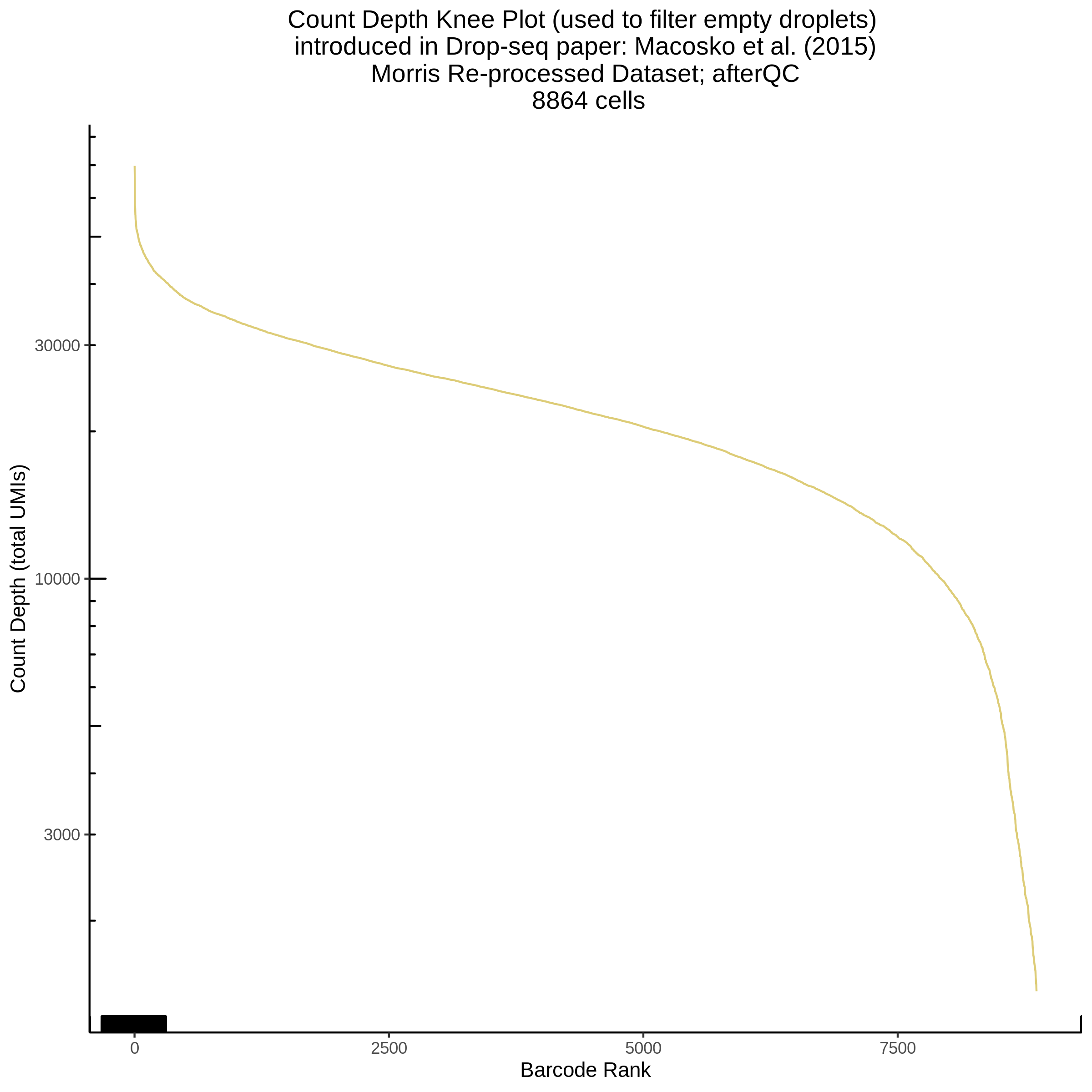
This is meant to be used in supplment to the plot above, where we
seek to define a lower bound for total UMI counts (count depth) based on
the distribution present in the data. 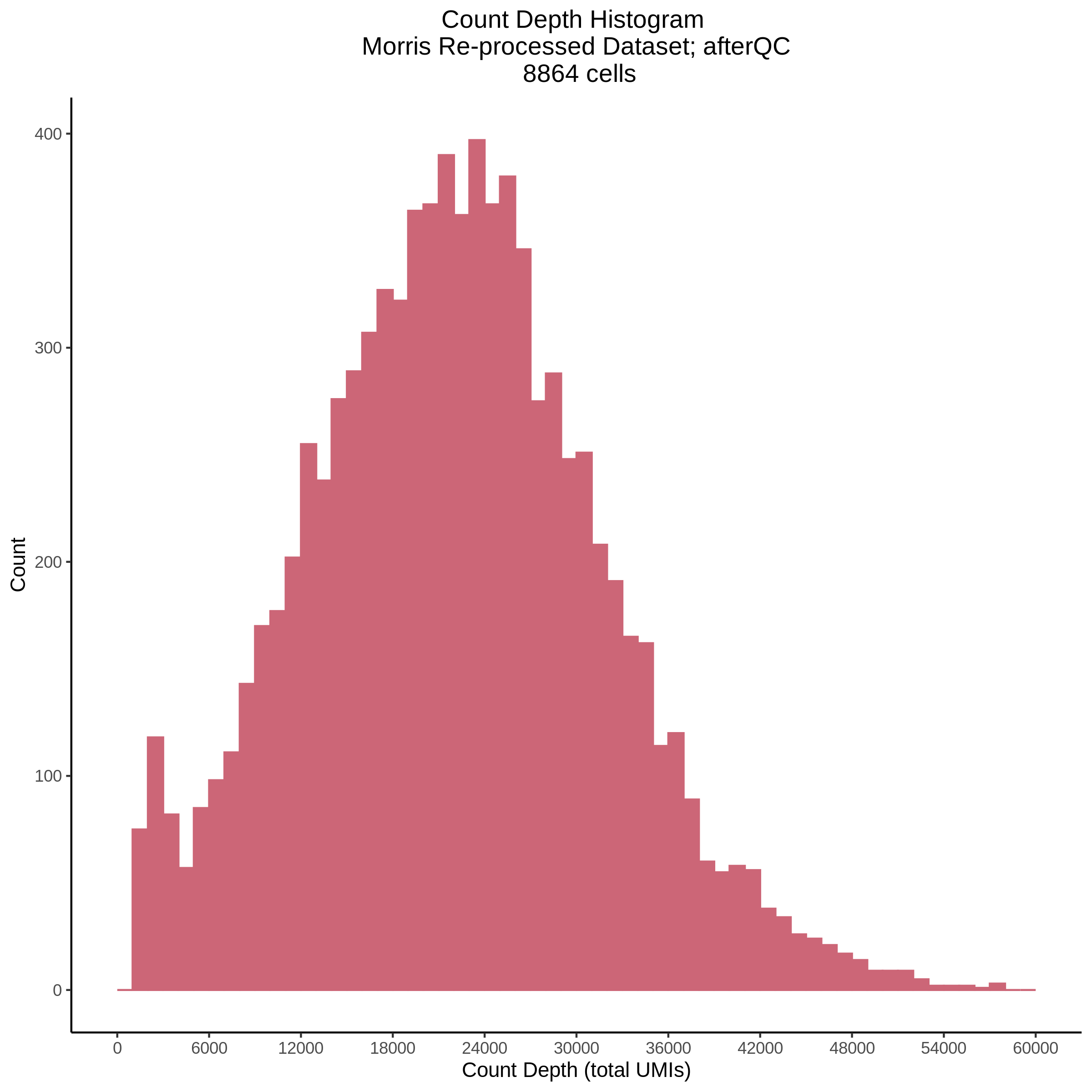
This plot is a scatter plot of count depth vs number of genes per
cell. This plot was taken from “Current best practices in scRNA-seq
analysis: a tutorial” Luecken & Theis. 2019 and to shows all cells
in the datasets as points. 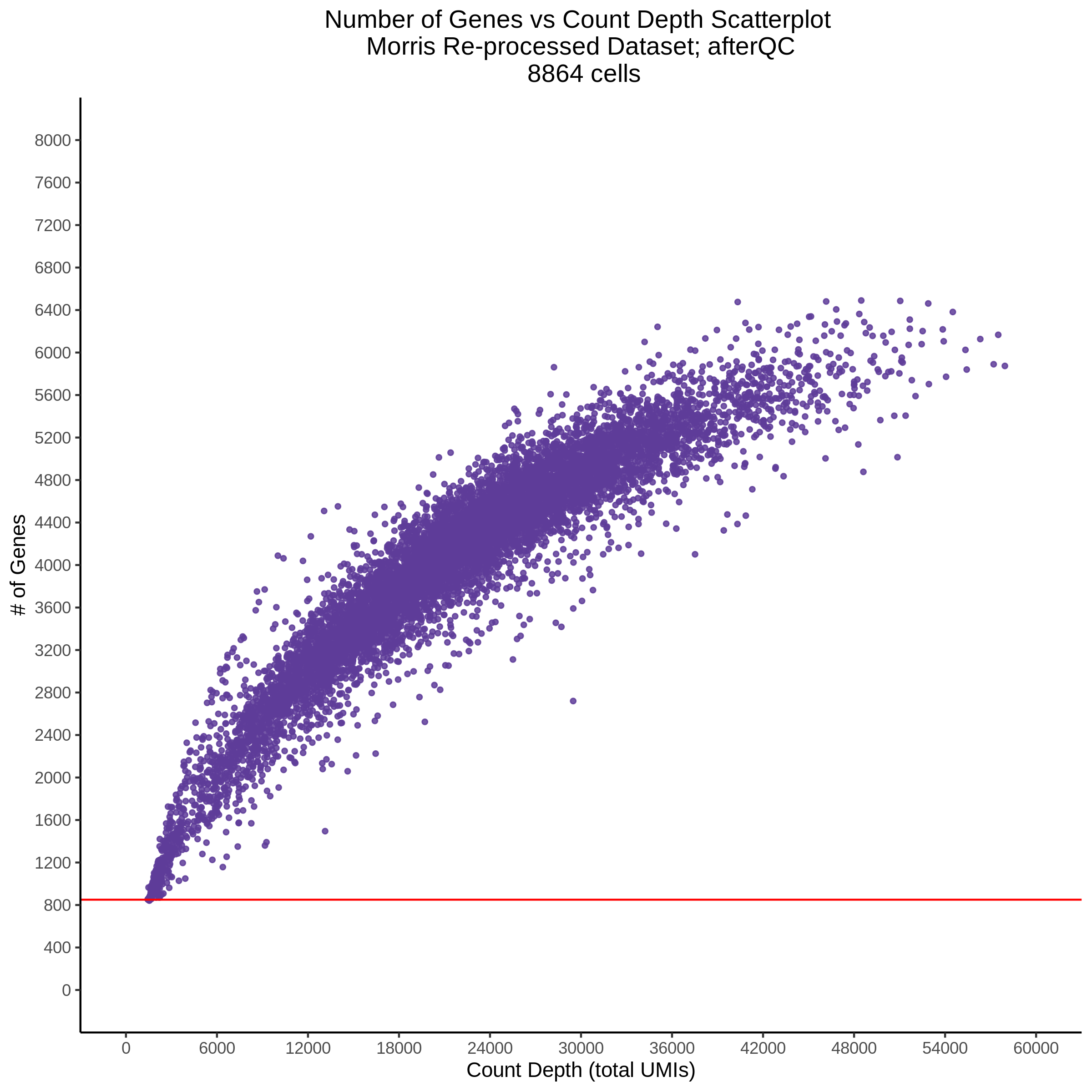
This is the canonical MOI plot or gRNA per cell plot. A red line is
placed on the median gRNAs per cell. 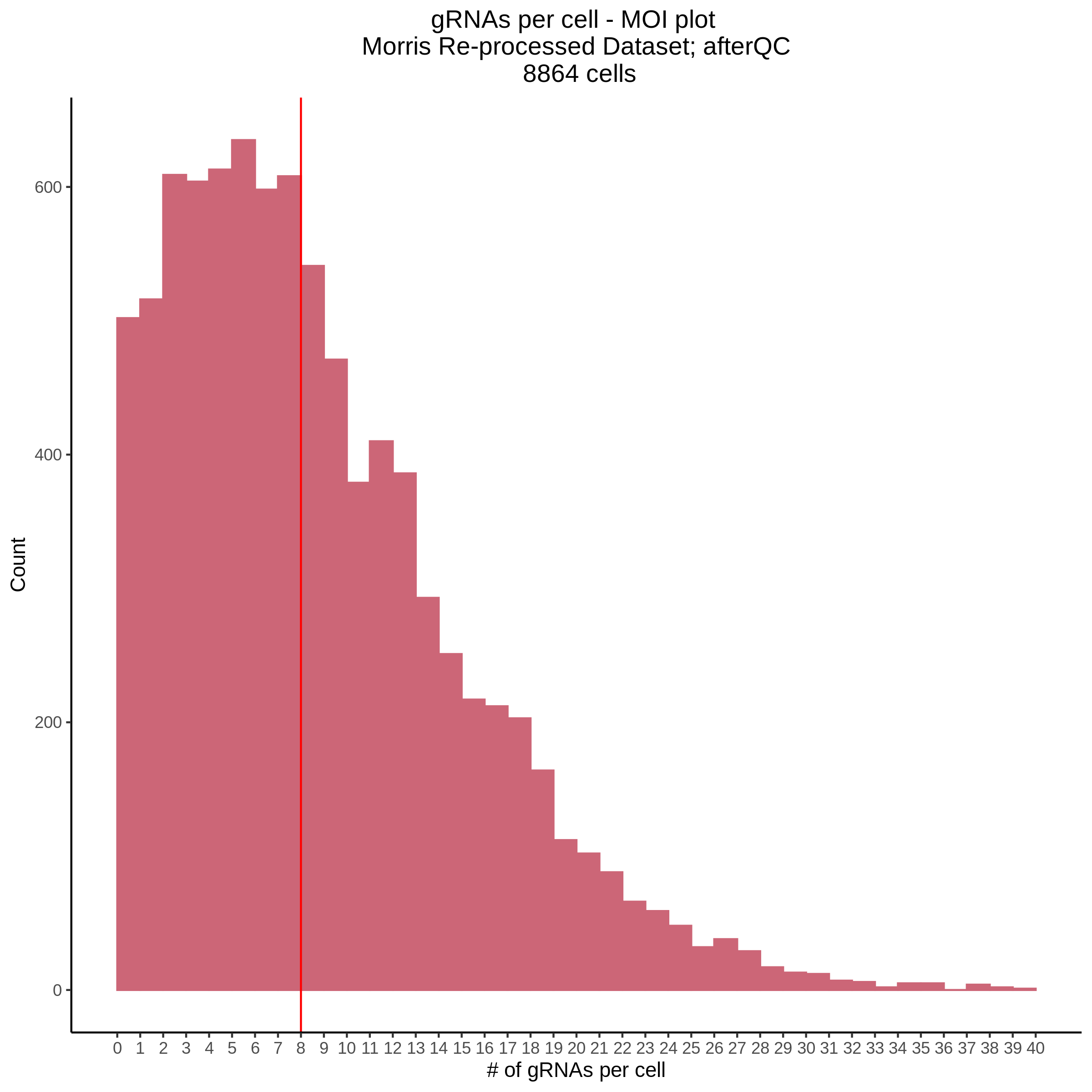
7/13/2022 Morris GEO Dataset QC
When looking at the UpsetR plots showing the intersection between significant gene-gRNA pairs between the Morris GEO dataset based SCEPTRE analysis and the re-processed raw data based analysis we saw that there was little overlap. This was cause for concern since we expect most of the results between the two to be the same. In order to investigate what is going on we will look at the QC thresholds and QC plots in both the GEO dataset and the re-processed dataset.
GEO Dataset
This dataset is taken directly from GEO: Morris GEO Dataset. GEO describes the dataset there as: “Processed data provided in standard UMI count matrix format for cDNA, GDO and HTO. Each sample has three files separated into features, barcodes and a sparse matrix file.”. Afterwards the data matrixes are pre-processed in order to apply QC thresholds and prepare the data for SCEPTRE analysis (input) within the general Snakemake pipeline.
GEO Dataset ALL cells
Plot of distribution of cells per gene as a histogram. 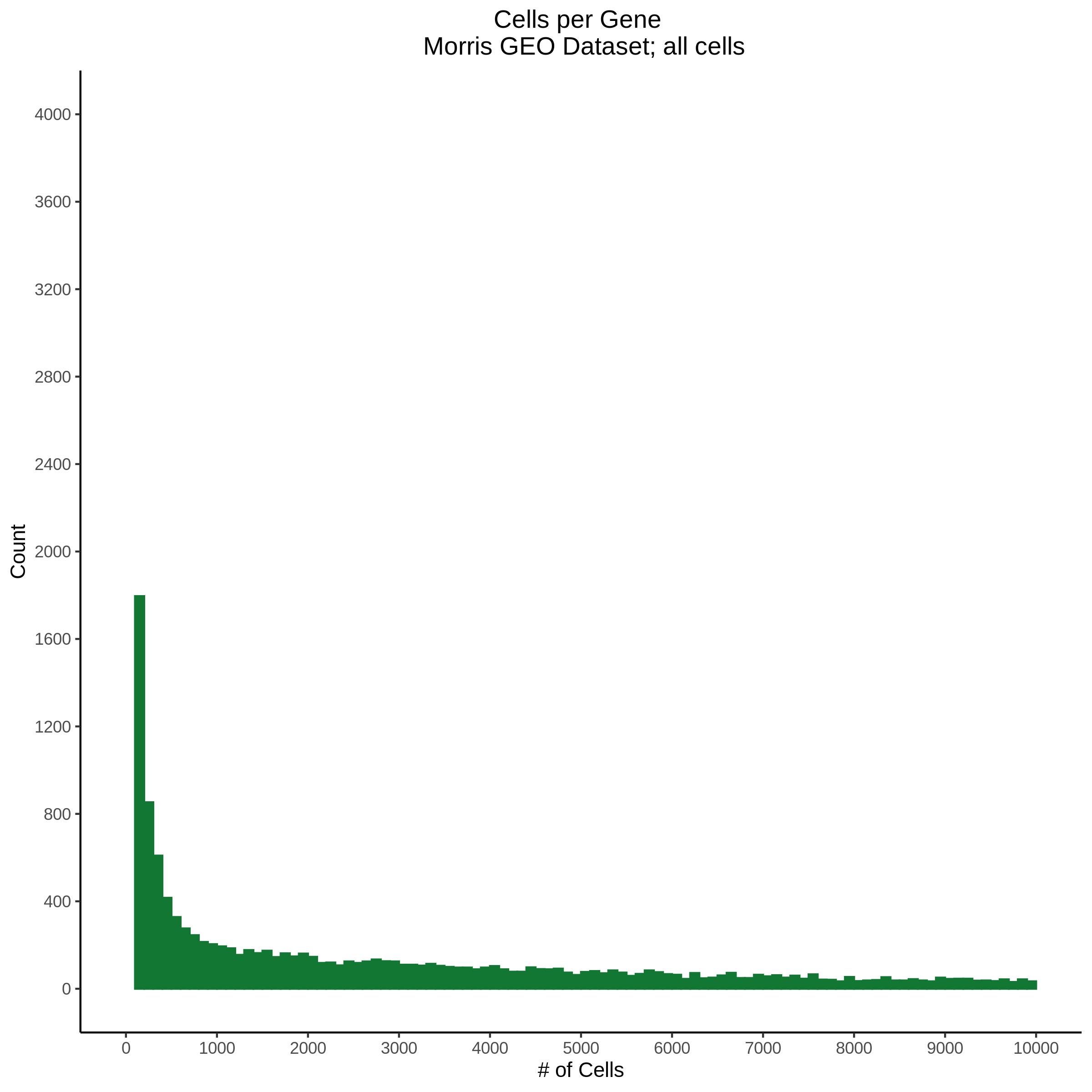
Plot of the distribution of genes per cell as a histogram. The y-axis
is in log10 becuase of the large amount of zeros when all cells are
considered. A red line is placed at the current QC threshold of 850
unique genes. 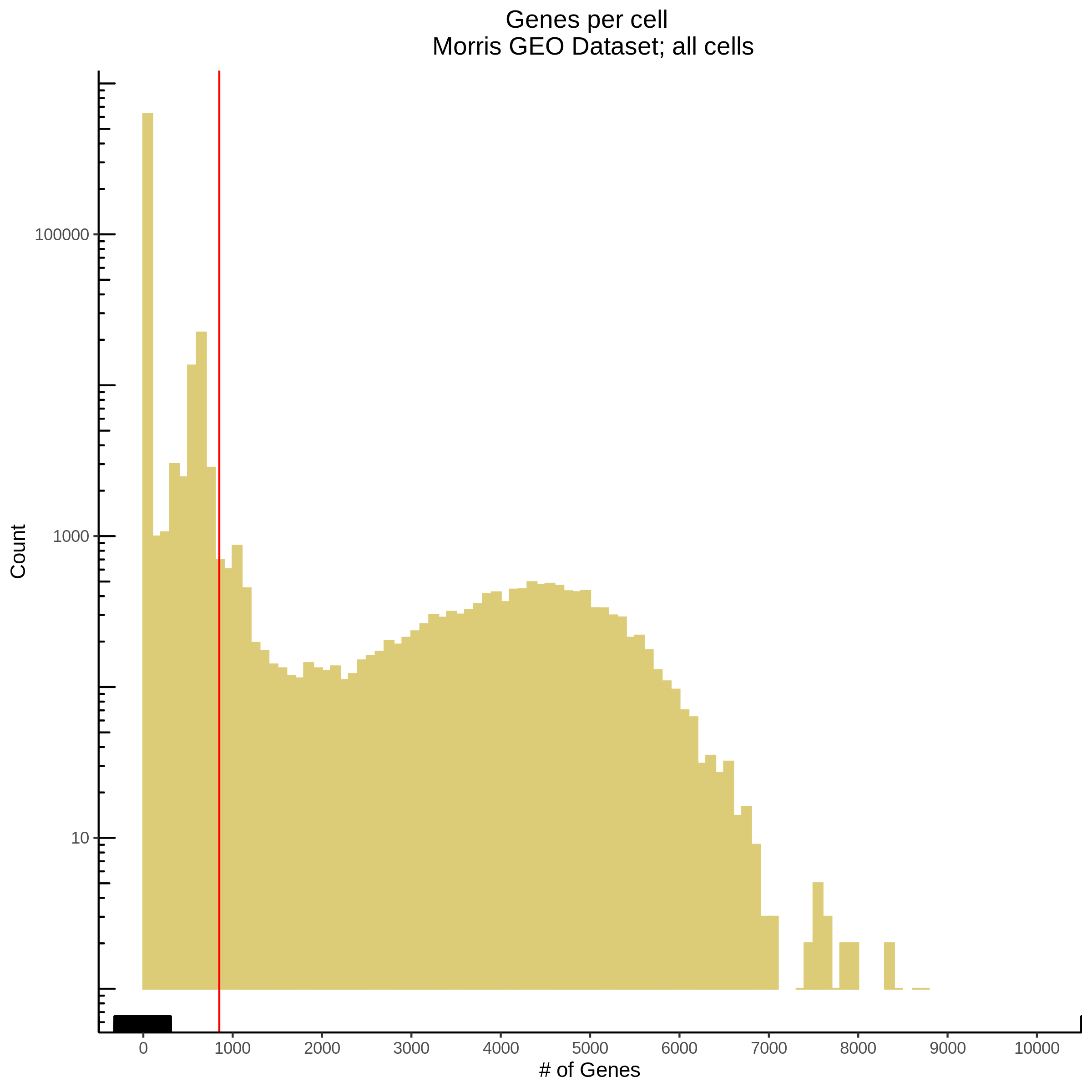
Plot of the count depth vs rank. The plot itself was introduced
originally in the Drop-seq paper (Macosko et al., Highly parallel
genome-wide expression profiling of individual cells using nanoliter
droplets, 2015.) Here you rank cells based on count depth to produce a
count depth (total UMIs) vs barcode rank plot and place a horizontal
threshold where the line curves down steeply. 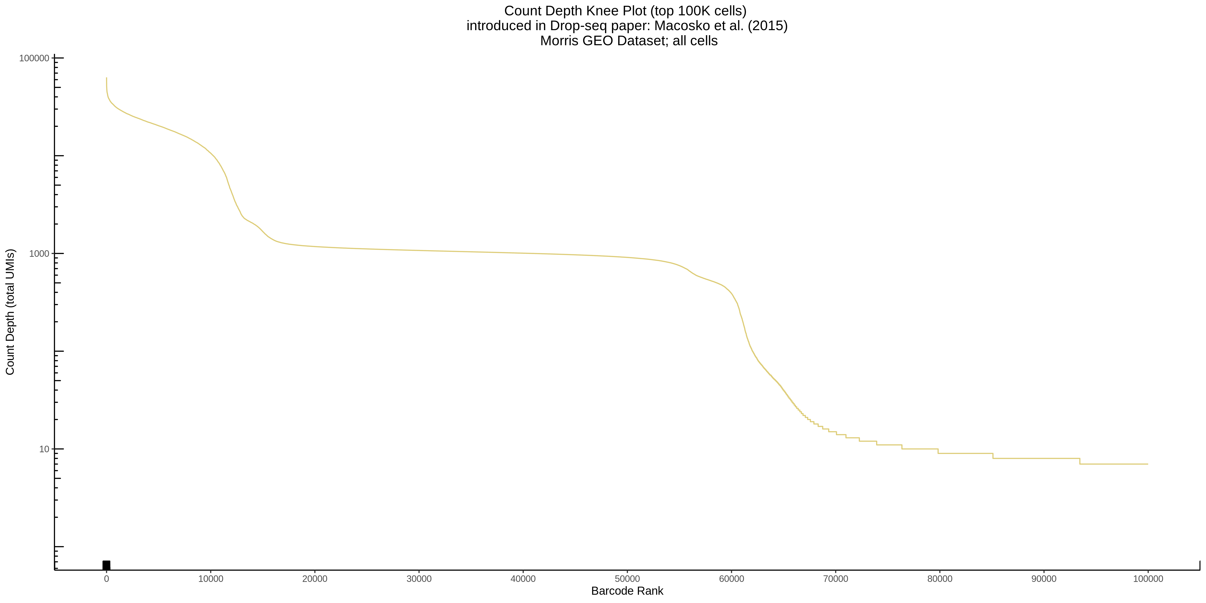
This is meant to be used in supplment to the plot above, where we
seek to define a lower bound for total UMI counts (count depth) based on
the distribution present in the data. This plot also features a log10
y-axis becuase of the sheer amount of zeros. 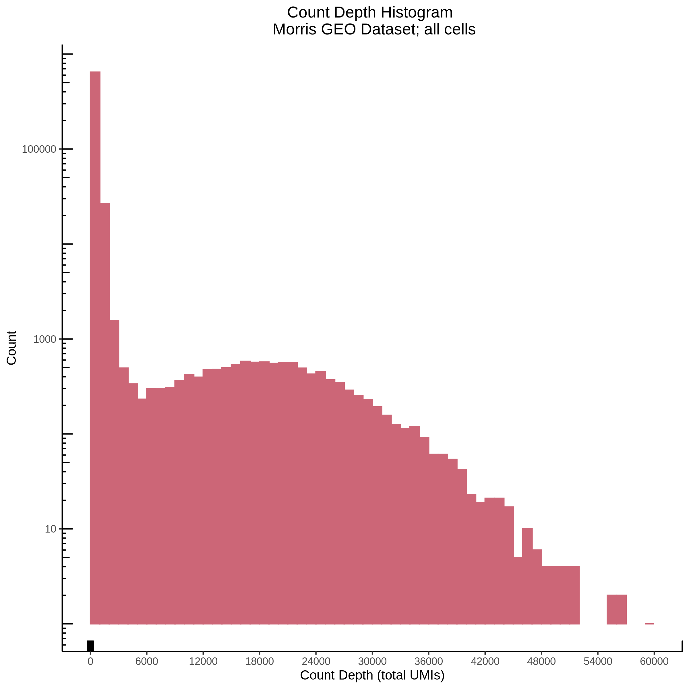
This plot is a scatter plot of count depth vs number of genes per
cell. This plot was taken from “Current best practices in scRNA-seq
analysis: a tutorial” Luecken & Theis. 2019 and to shows all cells
in the datasets as points. 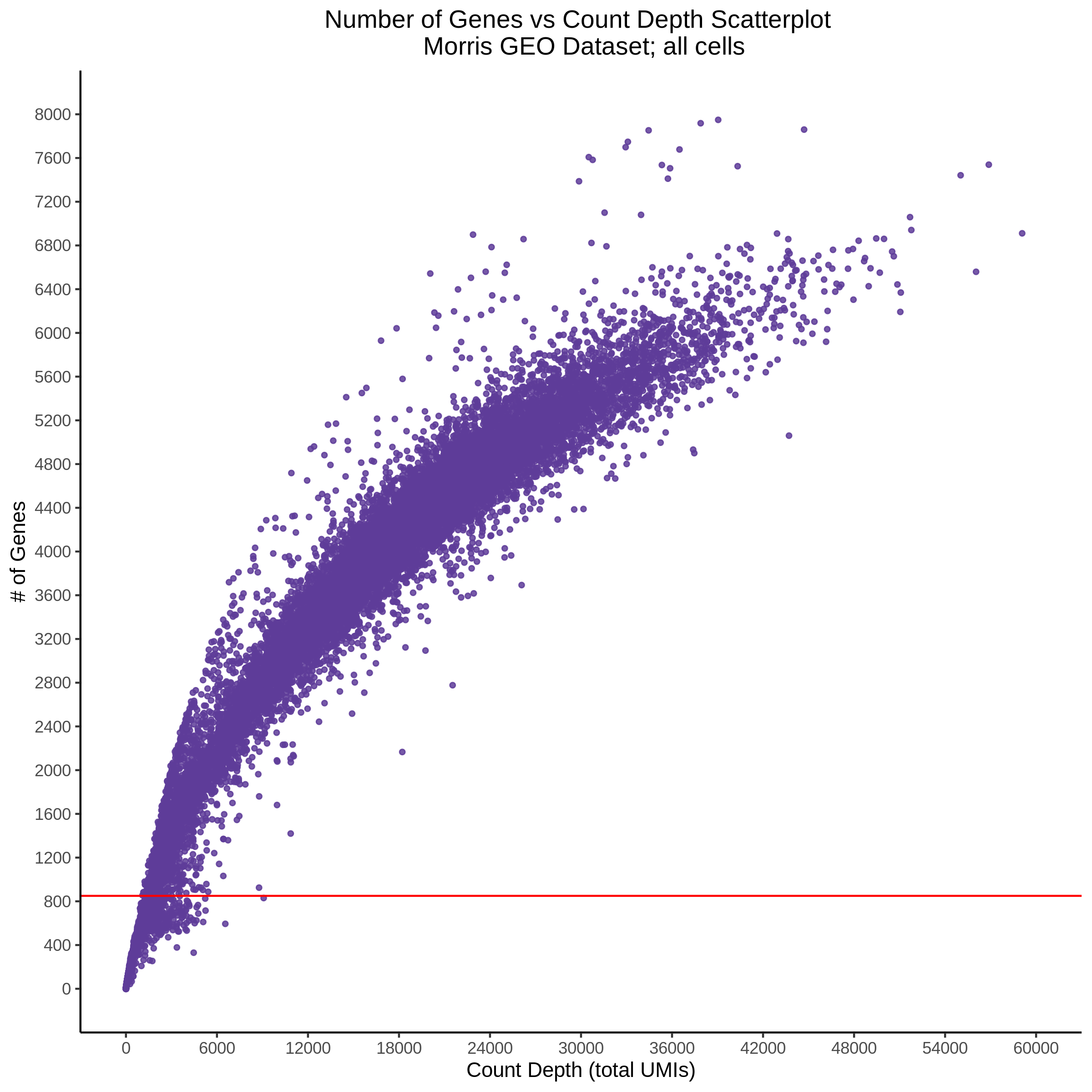
GEO Dataset post-QC
The point of this section is to illustrate that current QC thresholds as specified in the Morris manuscript are insuficient for the dataset on GEO. Here we replot the plots from above, adding in MOI, in order to show the distribution after QC. In places were applicable red lines have been added to show the location of a QC threshold.
For both the plots featuring count depth (total UMIs) there is no current (lower) threshold placed as it was not included in the manuscript. For that reason, these plots have no red line. I suspect that reason behind this was the use of the HTO matrix, which was used in conjuction with Suerats HTODemux function in order to identify singlets/multiplets/empty cells.
Plot of distribution of cells per gene as a histrogram. A red line is
placed at 5% of 9343 cells (467.15) as the minumum amount of cells a
gene must be found in, in order for it to be kept in the analysis. This
is used to filter out genes that are not found in most of the dataset
and that gene is not used later in association testing. 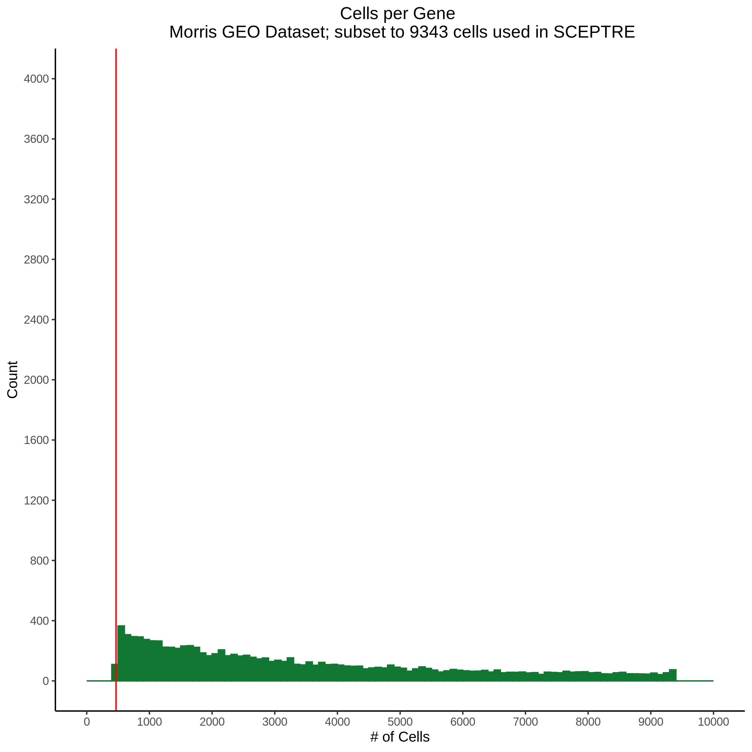
Plot of the distribution of genes per cell as a histogram. The y-axis
is frequency or count. A red line is placed at the current QC threshold
of 850 unique genes. 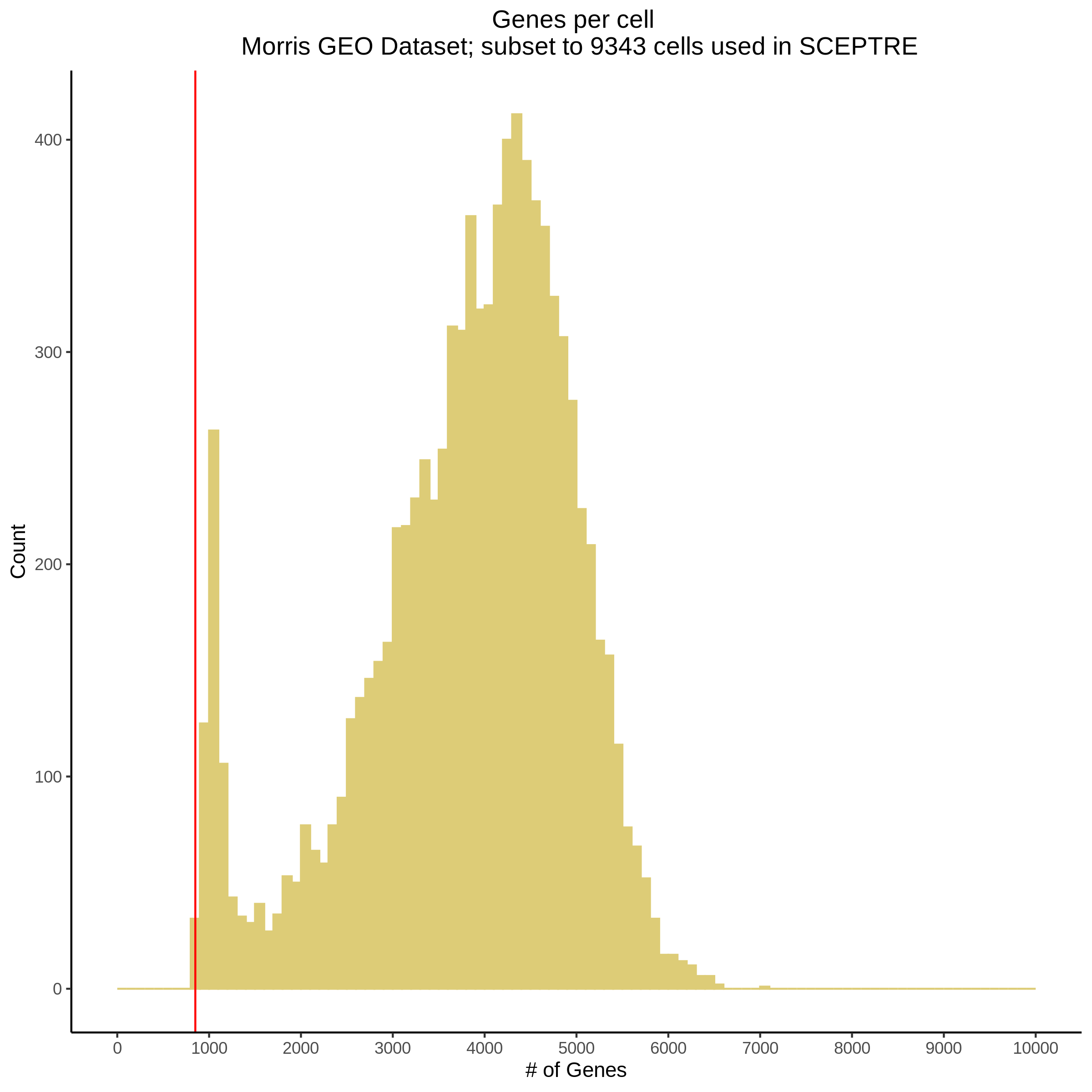
Plot of the count depth vs rank. The plot itself was introduced
originally in the Drop-seq paper (Macosko et al., Highly parallel
genome-wide expression profiling of individual cells using nanoliter
droplets, 2015.) Here you rank cells based on count depth to produce a
count depth (total UMIs) vs barcode rank plot. 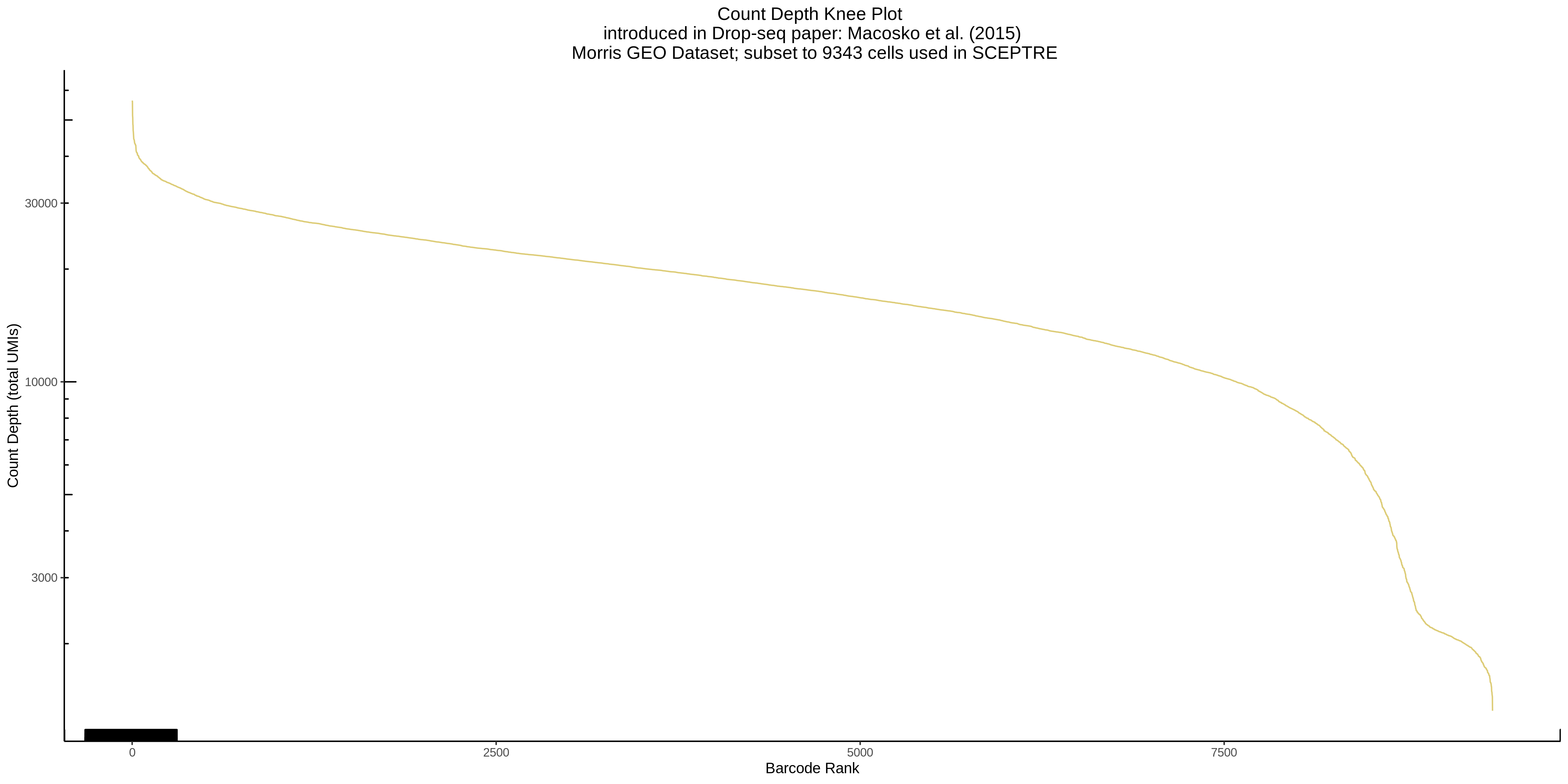
This is meant to be used in supplment to the plot above, where we
seek to define a lower bound for total UMI counts (count depth) based on
the distribution present in the data. 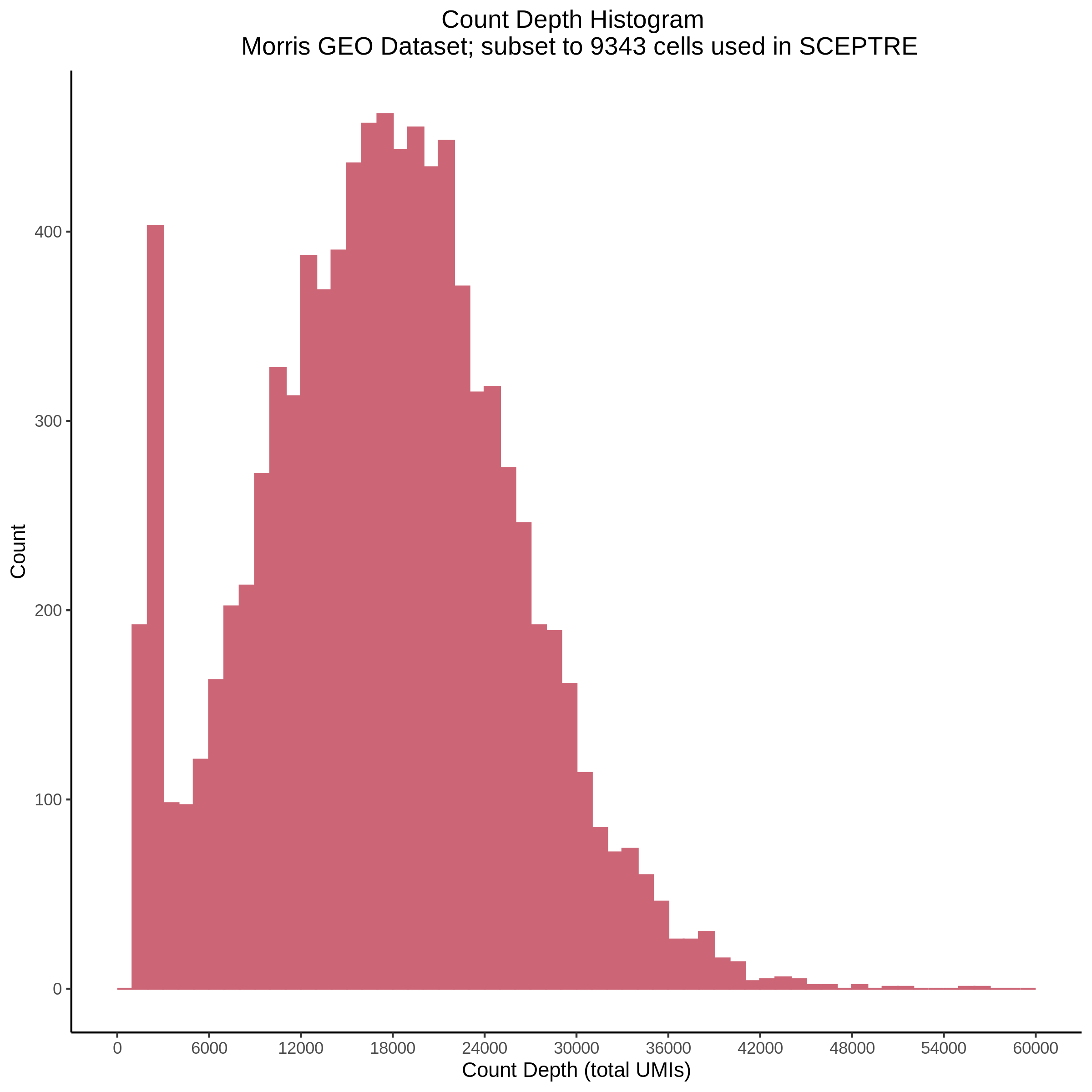
This plot is a scatter plot of count depth vs number of genes per
cell. This plot was taken from “Current best practices in scRNA-seq
analysis: a tutorial” Luecken & Theis. 2019 and to shows all cells
in the datasets as points. 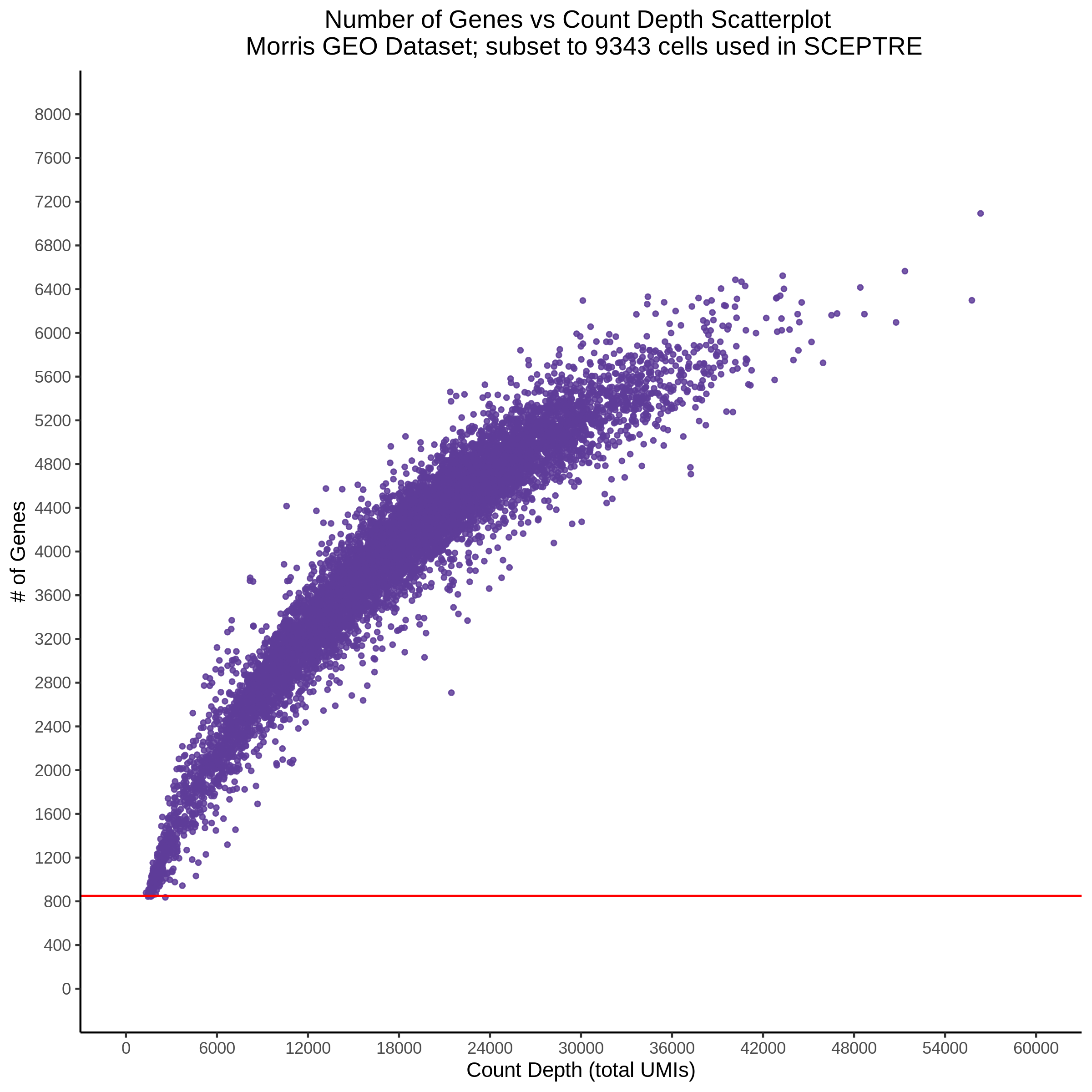
This is the canonical MOI plot or gRNA per cell plot. 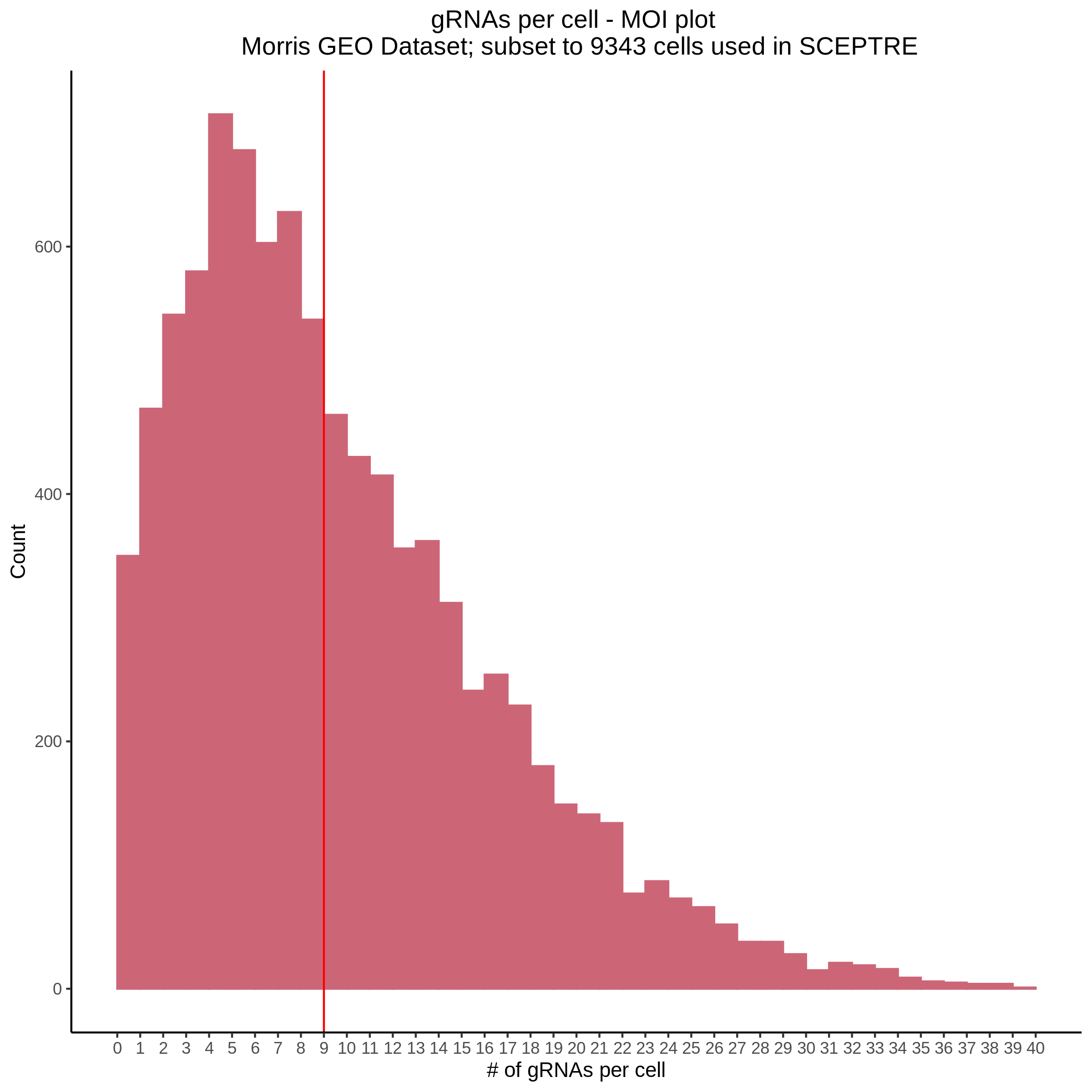
7/7/2022 Xie et al Data & QC
Introduction to dataset
Firstly, the Xie et al data set contains roughly 105k cells. The experiment is a CRISPR based scRNA seq by design. For this dataset, there are 5,170 sgRNAs targetting 516 enchancers. There are 10 sgRNAs per enchancer for a total of ~ 5,160 enchancer-sgRNAs and 10 control sgRNAs (6 NTCs, 4 PTCs?).
Cellranger Chemistry and Setup
The chemistry used for the library prep was 10X 3’ prime version 2. Prior to running cellranger on the raw data, we first look at the structure of the libraries sequenced to generate the data in the first place. Looking at the S2 Supplement table we see:
- RX196 10X K562-dCas9-KRABL2(Bai Lab) batch 1
- RX197 10X K562-dCas9-KRABL2(Bai Lab) batch 1
- RX212 10X K562-dCas9-KRABL2(Bai Lab) batch 2
- RX213 10X K562-dCas9-KRABL2(Bai Lab) batch 2
- RX216 10X K562-dCas9-KRABL2(Bai Lab) batch 3
- RX217 10X K562-dCas9-KRABL2(Bai Lab) batch 3
- DAA42 10X K562-dCas9-KRABL2(Bai Lab) batch 4
- DAA43 10X K562-dCas9-KRABL2(Bai Lab) batch 4
- RX224 10X K562-dCas9-KRABL2(Bai Lab) batch 5
- RX225 10X K562-dCas9-KRABL2(Bai Lab) batch 5
We can see that there are a total of 10 scRNAseq libraries over 5 batches. Initially, cellranger count was run on each batch (joining libraries) and then cellranger aggregate was used to correct for batch effects and merge UMI counts across all samples (single filtered matrix out). This was later changed to performing cellranger count on each library and then aggregating all counts into a single matrix.
6/28/2022 Morris Mappability-SCEPTRE Comparison Summary
Summary of Results
Below is a table of significant results. The adjusted p value threshold used was 5%.
| type | num_fdr_sig | num_bonf_sig |
|---|---|---|
| SNP | 802 | 196 |
| PTC | 76 | 38 |
| SNP-Mappability | 507 | 162 |
| PTC-Mappability | 32 | 15 |
Table of % Cross-Mappable Genes in Signals
Below is a table showing the percent of crossmapping significant results in each category. Each significant gene-gRNA pair is compared to a list of cross mapping genes (symmetric cross mappability score > 0). See 5/12 notes for details on how this was done.
| type | num_fdr_sig | num_bonf_sig |
|---|---|---|
| SNP | 0.7206983 | 0.6887755 |
| PTC | 0.8421053 | 0.8947368 |
| SNP-Mappability | 0.5621302 | 0.5493827 |
| PTC-Mappability | 0.8125000 | 0.8000000 |
UPSETR Plots for SNP targetting gRNAs between the old, geo dataset and the re-processed dataset.
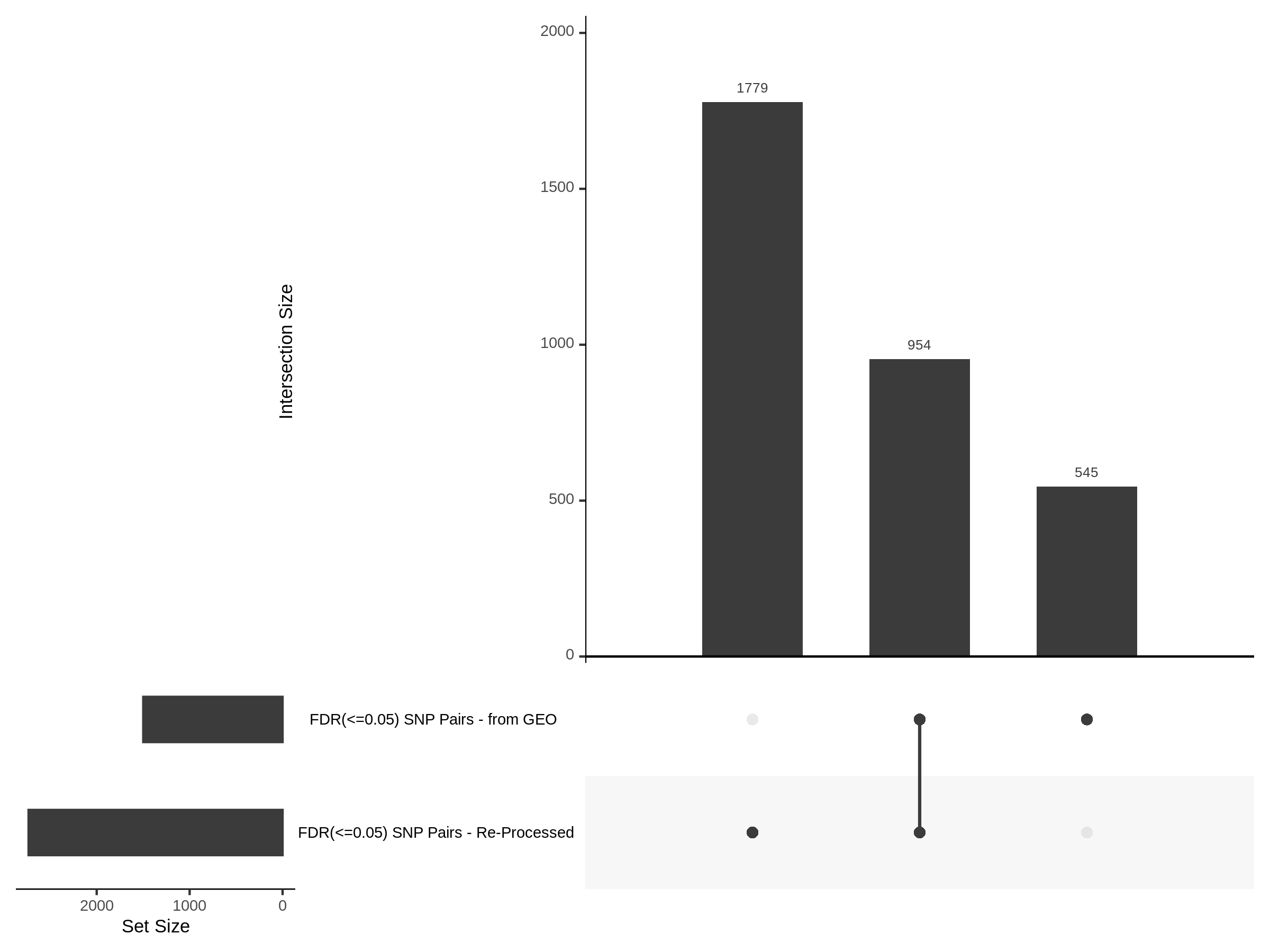
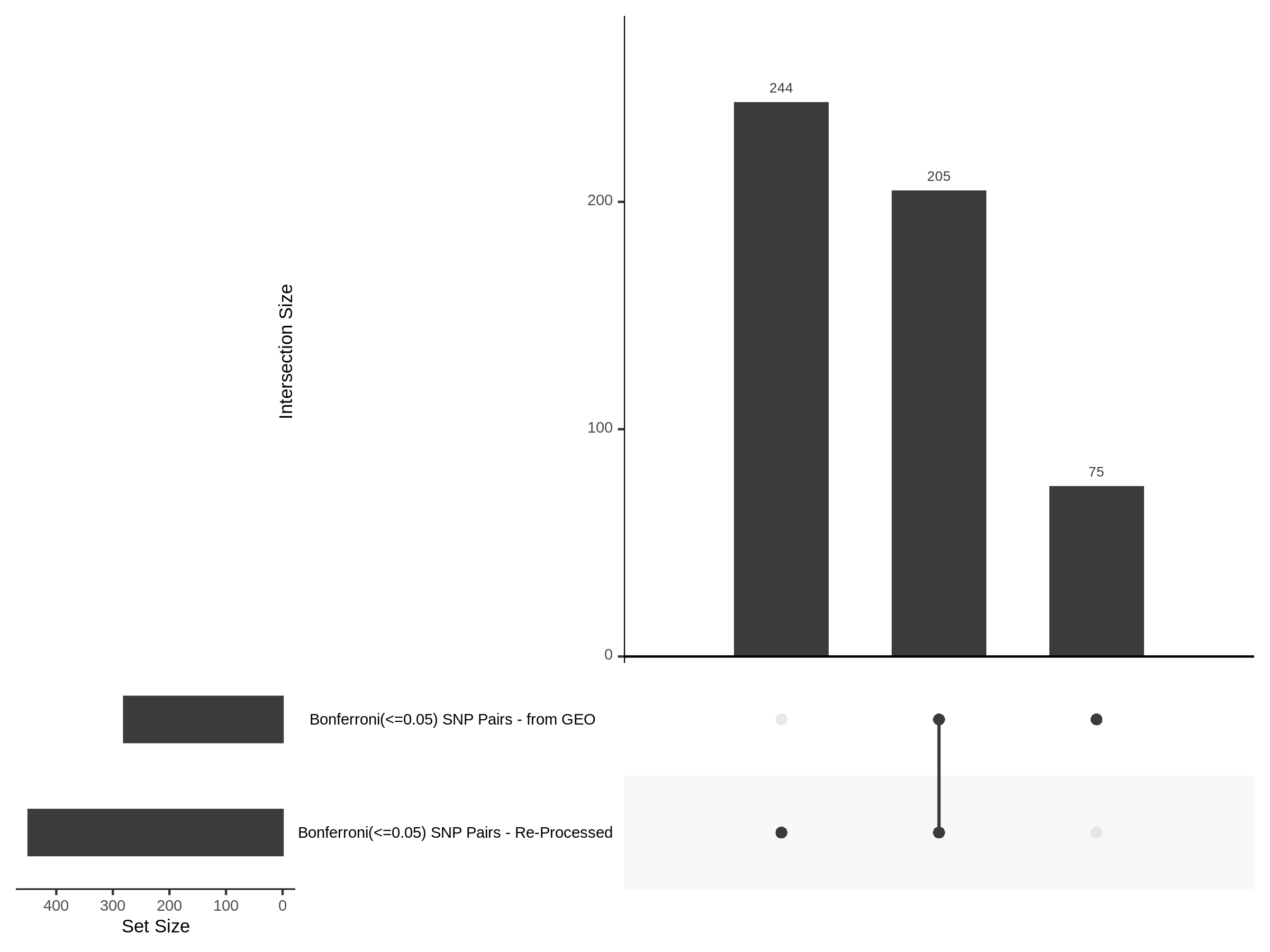
UPSETR Plots for PTC targetting gRNAs between the old, geo dataset and the re-processed dataset.
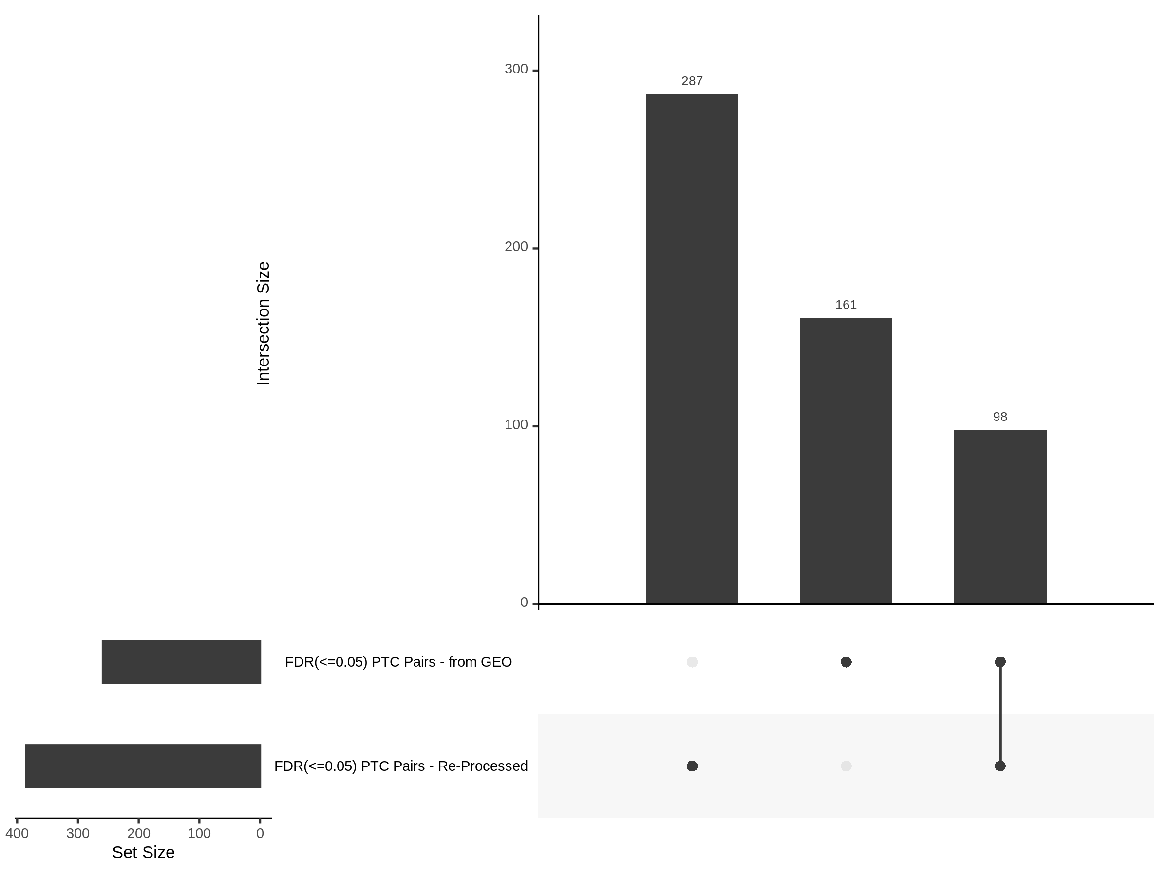
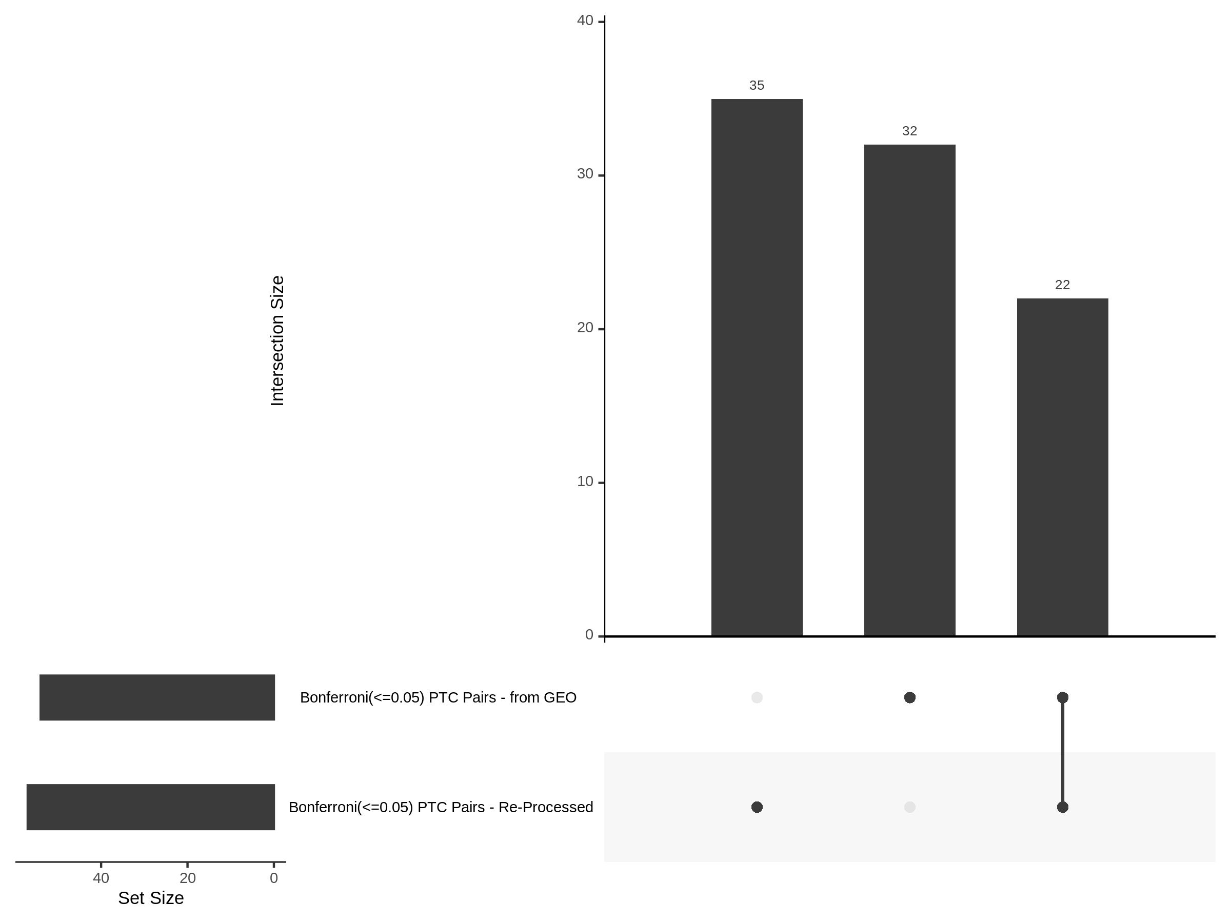
UPSETR Plots for SNP targetting gRNAs between the re-processed dataset and the mappability adjusted dataset.
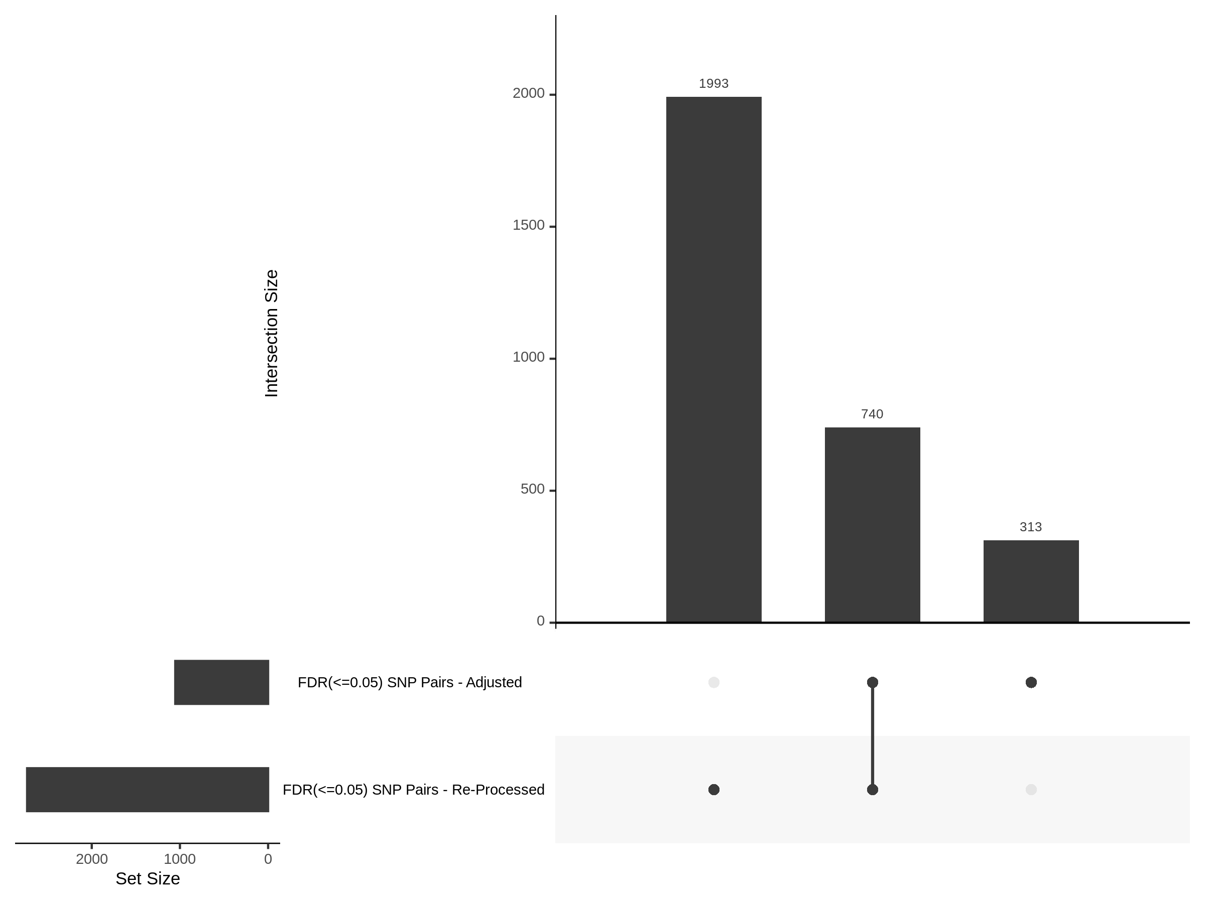
UPSETR Plots for PTC targetting gRNAs between the re-processed dataset and the mappability adjusted dataset.
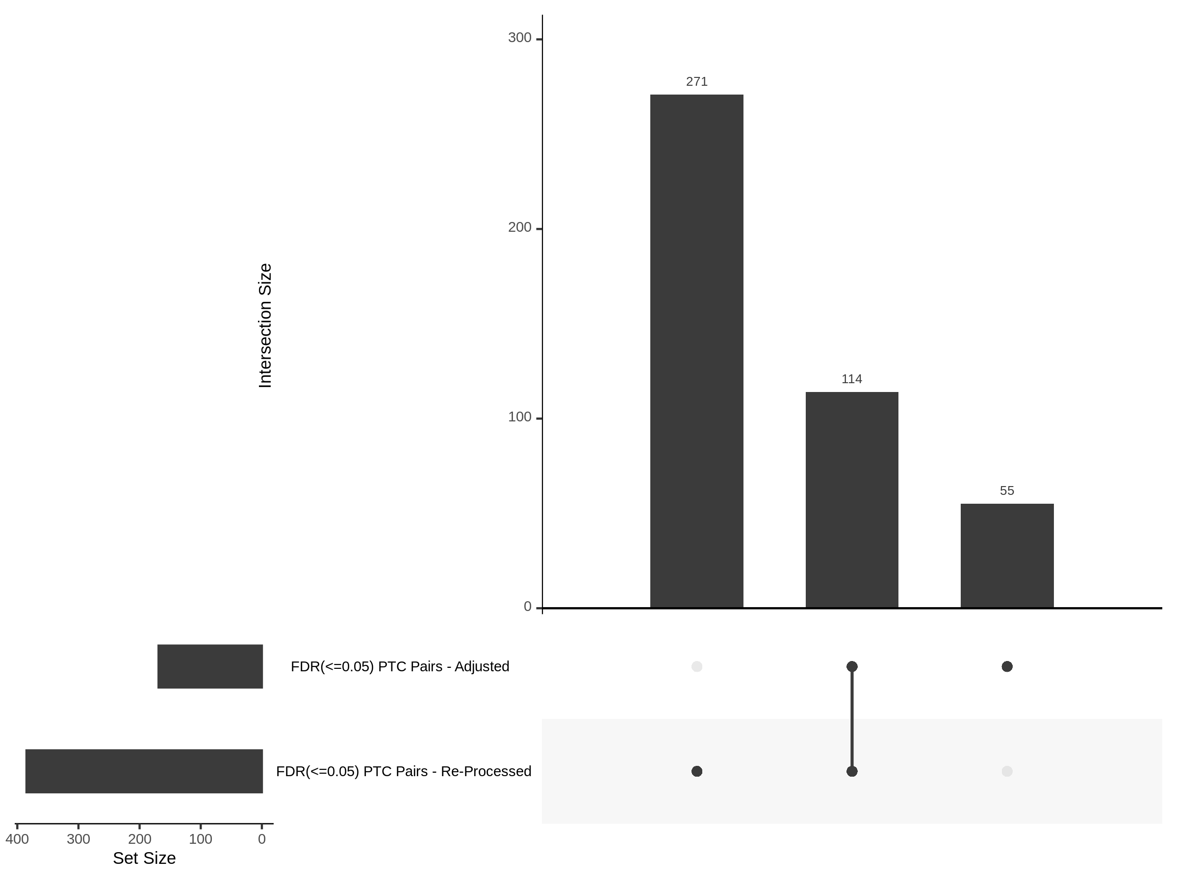
6/28/2022 Morris Mappability-SCEPTRE QQ Plots
QQPlots for Morris 2021 (NORMAL):
The general idea for this section is to check the NTC qqplots and histograms for the normal or un-adjusted SCEPTRE trans-analysis of the Morris dataset. The QCs used are shown below and SCEPTRE was run on pairs generated from the genes/gRNAs in the dataset. Each pair has a distance of at least 10Mb.
Expand NTC1
Expand NTC2
Expand NTC3
Expand NTC4
Expand NTC5
Expand NTC6
Expand NTC8
Expand NTC9
Expand NTC10
Expand NTC11
Expand NTC12
PTC pairs QQPlot
![]()
SNP pairs QQPlot
![]()
QQPlots for Morris 2021 (mappability adjusted):
The general idea for this section is to check the NTC qqplots and histograms for the mappability-adjusted SCEPTRE trans-analysis of the Morris dataset. This is a mirror run of the normal analysis with the only change being the GTF reference.
Expand NTC1
Expand NTC2
Expand NTC3
Expand NTC4
Expand NTC5
Expand NTC6
Expand NTC8
Expand NTC9
Expand NTC10
Expand NTC11
Expand NTC12
Adjusted PTC pairs QQPlot
![]()
Adjusted SNP pairs QQPlot
![]()
6/15/2022 CellRanger + QC
The main objective of this section is to describe how raw data from scRNA seq experiments, such as Morris 2021, Gasperini 2019, and Xie 2019, are run through the CellRanger pipeline and QC in the context of our mappability paper/test.
Preprocessing or alignment is relatively straightforward. cDNA reads (usually in R2 of the fastq files) from transcripts are split into groups according to cells, based on cell barcodes (usually R1), and then aligned to a reference to determine molecules of origin. The aligned reads are then collapsed based on UMI (usually R1). Collapsing is done because during PCR there might be PCR duplicates that are from the original transcript. In order to only count each unique transcript once, a collapsing strategy must be used prior to counting. Typically, this is done solely based on UMI and cDNA aligned to genes. For example, the collapsing strategy used by kallisto | bustools and applicable to droplet-based methods is the following:
- Group reads based on cell barcodes with a hamming distance = 1.
- Align reads
- All reads that have identical UMI, aligned to the same gene in step 2), are PCR duplicates
- Collapse UMIs
- Generate a gene by cell UMI count matrix based on 4) and 1)
This is known as the naïve approach to collapsing UMIs and allows for computational efficiency since it forms the problem of collapsing into a NP problem, as opposed to NP complete alternative. This is partially why Kallisto is near-optimal. Cellranger uses a similar workflow, and its only major difference is that alignment is not. In Cellranger, alignment is base-pair to the genome via STAR/STARsolo while Kallisto uses pseudoalignment to the refence transcriptome to generate count matrixes. Cellranger also uses the same hamming distance of 1 to correct cell barcodes in step 1) above, in fact, Kallisto borrowed this step from Cellranger.
Raw data: Typically, data from scRNA seq perturbation experiments (scRNAseq + CRISPR) using 10x Chromium technology is reported in paired fastq files, labeled based on lane arising from each Chromium device (GEM wells). This is because each lane in a Chromium Device is expected to process up to 10,000 cells per lane. For example, data from Morris 2021 is reported on GEO as the following:
- cDNA1_S1_L001_R1_001.fastq
- cDNA1_S1_L001_R2_001.fastq
- cDNA1_S1_L002_R1_001.fastq
- cDNA1_S1_L002_R2_001.fastq
- cDNA2_S1_L001_R1_001.fastq
- cDNA2_S1_L001_R2_001.fastq
- cDNA2_S1_L002_R1_001.fastq
- cDNA2_S1_L002_R2_001.fastq
- cDNA3_S1_L001_R1_001.fastq
- cDNA3_S1_L001_R2_001.fastq
- cDNA3_S1_L002_R1_001.fastq
- cDNA3_S1_L002_R2_001.fastq
- cDNA4_S1_L001_R1_001.fastq
- cDNA4_S1_L001_R2_001.fastq
- cDNA4_S1_L002_R1_001.fastq
- cDNA4_S1_L002_R2_001.fastq
From this we see that there are 4 samples using 2 lanes of a single
GEM well. We can aggregate samples within a GEM well for quantification.
We can then run the cellranger count pipeline (assuming we have valid
cellranger references made). For larger datasets each GEM well needs to
be run separately and the final cellranger count output aggregated using
cellranger’s aggregation function (cellranger agg -h).
After running cellranger count pipeline, we can proceed to performing QC
on the outputted filtered_feature_bc_matrix folder containing our gene
by cell matrix in MTX format.
Summary of QC: We apply a few QC thresholds.
- Cells with mitochondrial ratio/percent less than <= 0.2/20%
- Genes expressed in at least 5% of all cells
- gRNAs expressed in at least 50 cells (retains a majority of gRNAs)
- Cells with at least 850 unique gene UMIs
- Cells with at least one HTO and less than 2500 total HTO counts (only applicable to datasets w/ HTO data)
The resulting gRNA (perturbation) and cDNA (expression) matrixes are feature by cell, and are used as inputs for SCEPTRE analysis.
How does this process fit into the overall experiment?
The point of having a unified, snakemake, pipeline for processing raw scRNAseq cDNA expression data into UMI count matrixes is because our method for improving trans gene regulation with SCEPTRE relies on carefully modifying the quantification step. As outlined above, we can see that aligning reads to the reference is done prior to collapsing UMIs and counting them. Our method introduces a modified reference into this step specifically. We modify the reference GTF annotation used to construct the cellranger reference by removing low mappability regions. The adjusted reference is then used to quantify gene expression in a more conservative way, as we hope to improve detecting trans regulatory signals by removing regions that are problematic in the alignment step due to the multi mapping issue. Thus, the snakemake pipeline insures that our treatment of the cDNA expression data remains the same throughout the experiment with respect to all quantification and quality control steps.
5/12/2022 Signals and Cross-Mappability
In order to begin investigating which signals from SCEPTRE trans analysis are cross mappable, we took the signifcant gene-gRNA pairs and intersected them with genes identified as being cross-mappable based on a Symmetric Cross-Mappabiity score from False positives in trans-eQTL analysis arising from RNA seq alignment errors.
First data from the above paper was downloaded; notably two versions corresponding to the hg19 and hg38 references. Both sets use a kmer length = 76 for exonic regions and a kmer=36 for UTR regions. This represents a region of 76 mers from the genes exonic regions and 36 mers from its untranslated regions with a maximum tolerance of 2 mismatches.
Terms:
- Cross-mappability from gene A to gene B, crossmap(A,B), is defined as the number of gene A’s k-mers whose alignment start within exonic or untranslated regions of gene B.
- Symmetric Cross-mappabiity between gene A and gene B is defined as (crossmap(A,B) + crossmap(B,A))/2.
The data for symmetric cross-mappability is a 3 column table, with the first two columns defining gene A and gene B, and the last column being the symmetric cross-mappabiity. The genes are originally reported using ENSEMBL ids, which match our gene_id column in SCEPTRE results.
gene A              gene B              symmetric cross-mappabiity
ENSG00000000003.10  ENSG00000100058.8     25
ENSG00000000003.10  ENSG00000101017.9     5.5
ENSG00000000003.10  ENSG00000102595.14  8
After intersection we can classify our results using a binary flag: cross_maps; which indicates if a gene in a gene-gRNA pair has a non-zero symmetric cross-mappability score (TRUE/FALSE). The table below is based on the significant table from 4/28 (below).
Morris 2021
| site_type | bh_reject (FDR=<0.05) pairs w/ symmetric cross-mapping | bh_reject (FDR=<0.05) pairs (cross-map = FALSE) | bonferroni_reject (=<0.05) pairs w/ symmetric cross-mapping | bonferroni_reject (=<0.05) pairs (cross-map = FALSE) | total bh_reject (FDR=<0.05) | total bonferroni_reject (=<0.05) |
|---|---|---|---|---|---|---|
| SNP | 445 | 169 | 124 | 52 | 614 | 176 |
| PTC | 131 | 22 | 53 | 4 | 153 | 57 |
Gasperini 2019
| site_type | bh_reject (FDR=<0.05) pairs w/ symmetric cross-mapping | bh_reject (FDR=<0.05) pairs (cross-map = FALSE) | bonferroni_reject (=<0.05) pairs w/ symmetric cross-mapping | bonferroni_reject (=<0.05) pairs (cross-map = FALSE) | total bh_reject (FDR=<0.05) | total bonferroni_reject (=<0.05) |
|---|---|---|---|---|---|---|
| DHS | 2245 | 1243 | 878 | 448 | 3488 | 1326 |
| TSS | 8494 | 3738 | 1370 | 572 | 12232 | 1942 |
5/11/2022 Checking NTC Inflation in Gasperini trans-wide SCEPTRE
We found that some gRNAs, NTCs, appeared to be inflated with p values deviating from expectation in the Morris tran-wide analysis. This is shown below on ‘4/20/2022 Morris trans-wide SCEPTRE NTC QQPlots’ wherein a few of the NTCs showed inflation while others did not. In order to investigate this further in another dataset, here we will plot NTC p values from the Gasperini 2019 trans-wide SCEPTRE analysis.
Gasperini 2019 SCEPTRE trans-wide: NTC Random_1
Gasperini 2019 SCEPTRE trans-wide: NTC Random_23
Gasperini 2019 SCEPTRE trans-wide: NTC Random_25
Gasperini 2019 SCEPTRE trans-wide: NTC Random_9
Gasperini 2019 SCEPTRE trans-wide: NTC Scrambled_1
Gasperini 2019 SCEPTRE trans-wide: NTC Scrambled_3
Gasperini 2019 SCEPTRE trans-wide: NTC Scrambled_25
5/4/2022 SCEPTRE Z-scores of NTCs
Updated on 5/11/2022:
This update includes additional investigation of the resampled statistics (z-scores) that are used to construct the emperical null distribution in SCEPTRE analysis. In order to further investigate we now plot a histogram of their p values (Z scores forming the null converted to p values using original SCEPTRE fit_t_skew(), which uses R selm in order to fit linear models with skew-elliptical error term)
The idea is to inspect the z scores of NTC pairs which are both normal-looking (non-significant, on expected line in qpplot) vs NTC pairs that showed p-value inflation.
First, we identify the NTC pairs we are interested in looking into. This is done by inspecting NTC pairs ordered by -log10(p_value) specific to a gRNA (NTC). From NTC plots by NTC on 4/20/2022, we see that NTC-8 shows a lot of inflation while NTC-4 and NTC-1 are relatively normal. Looking at just the expanded grid plot (which contains NTCs adjusted all-together) we see that by descending order points #5 on both NTC-1 and NTC-4 are almost exactly on the expected line with an observed -log10(p_value) value of about ~3.34/3.07, while descending point #1 on NTC-8 (as well as a few others) is inflated with an observed -log10(p_value) value of ~8.11.
We can pull out these 3 pairs with the corresponding information. The index column corresponds to rank by descending -log10(p_value). Based on above reasoning, we select #1 from NTC-8 and #5 from both NTC-1 and NTC-4.
idx  gene_id     gRNA_id    p_value  neglog10_obs_pval
 5 ENSG00000171045 NTC-1   0.000457               3.34
 5 ENSG00000110063 NTC-4   0.000849               3.07
 1 ENSG00000108298 NTC-8   0.00000000782              8.11

other pairs:
 2 ENSG00000171863 NTC-8   0.0000000154               7.81
 3 ENSG00000161016 NTC-8   0.0000000197               7.70
 4 ENSG00000110700 NTC-8   0.0000000235               7.63
 5 ENSG00000178741 NTC-8   0.0000000257               7.59
 1 ENSG00000101182 NTC-4   0.000202              3.70
 2 ENSG00000099901 NTC-4   0.000320              3.50
 3 ENSG00000145191 NTC-4   0.000343              3.47
 4 ENSG00000172977 NTC-4   0.000403              3.40
 1 ENSG00000100865 NTC-1   0.0000251              4.60
 2 ENSG00000215154 NTC-1   0.000214               3.67
 3 ENSG00000254093 NTC-1   0.000308               3.51
 4 ENSG00000173559 NTC-1   0.000309               3.51
Then we can then plot the resampled test statistics of these 3 gene-gRNA pairs.
Morris trans: NTC-1 Top 5 gene-gRNA pair resampled test statistics plot
Morris trans: NTC-1 Top 5 gene-gRNA pair resampled test statistics histogram
Morris trans: NTC-4 Top 5 gene-gRNA pair resampled test statistics plot
Morris trans: NTC-4 Top 5 gene-gRNA pair resampled test statistics histogram
Morris trans: NTC-8 Top 1 gene-gRNA pair resampled test statistics plot
Morris trans: NTC-8 Top 1 gene-gRNA pair resampled test statistics histogram
Additional plots:
Morris trans: NTC-1 Top 1 gene-gRNA pair resampled test statistics plot
Morris trans: NTC-1 Top 1 gene-gRNA pair resampled test statistics histogram
Morris trans: NTC-4 Top 1 gene-gRNA pair resampled test statistics plot
Morris trans: NTC-4 Top 1 gene-gRNA pair resampled test statistics histogram
Morris trans: NTC-8 Top 5 gene-gRNA pair resampled test statistics plot
Morris trans: NTC-8 Top 5 gene-gRNA pair resampled test statistics histogram
4/28/2022 Distribution of Pair Distances in Morris and Gasp. Transcriptome-wide Analysis
Briefly, in order to check trans pairs, the distance between each gene-gRNA pair was calculated for both the Morris and Gasperini pairs run in the SCEPTRE analysis. This was done by gettting the gene position infomation from the reference genome, and the position of gRNA target. This is availible for all gene-gRNA pairs tested. A additional flag value of -1 is used to indicate pairs across chromosomes. Below are the plotted distances seperated by site_type (SNP, PTC (TSS), TSS, and DHS pairs)
Morris 2021 gene-gRNA pair distances:
Morris 2021
Gasperini 2019 gene-gRNA pair distances:
Gasperini 2019
4/28/2022 Morris and Gasp. trans-wide Signal Summary Table
Originally made on 4/14/2022, this was updated to reflect a major correction. See day below.
Morris 2021 and Gasperini 2019 trans-wide Results:
Trans gene-gRNA pairs are defined as genes at least >=10Mb from the gRNA target.
| site_type | bh_reject (=<0.05) | bonferroni_reject (=<0.05) |
|---|---|---|
| SNP | 614 | 176 |
| PTC | 153 | 57 |
| site_type | bh_reject (=<0.05) | bonferroni_reject (=<0.05) |
|---|---|---|
| DHS | 3488 | 1326 |
| TSS | 12232 | 1942 |
4/28/2022 Morris and Gasp. trans-wide Analysis Significant Signals Tables
Originally 4/20/2022
This was updated in order to reflect changes/correction of mistate. 1) The trans pairs were not correct. 2) Gene-gRNA pairs included non-autosomal genes on MT,X,Y.
Here are links to tables containing significant results using two different corrections: + FDR (bh) <= 0.05 + Bonferroni <= 0.05
The Morris transcriptome-wide SCEPTRE results contain two types of pairs, SNP and PTC. The PTC pairs are made by pairing the positive controls targeting the TSS of genes such as CD42, CD52, and CD55.
The tables also contain addition columns.
- id: this is a unique id given to each pair tested
- site_type: this is used to distinguish SNP vs PTC pairs.
- rsID: this is the rsID of a SNP targeting pair (if the gRNA is a SNP type)
- SNP_info: this contains the condensed SNP positional info (if the gRNA is SNP type)
- SNP_closest_gene_TSS: this is the gene symbol of the gene closest to the SNP target region
- SNP_chr: chromosome the SNP is on
- SNP_location: SNP location on chr (see above)
- gene_chromosome_name: chromosome the gene is on (taken from the Ensembl 96 reference used in the preprint)
- gene_start_position: start of gene
- gene_end_position: end of gene
- gene_hgnc_symbol: gene symbol of gene in gRNA-gene pair
- PTC_ensembl_gene_id: gene id of PTC gene-gRNA pair, gene symbol is availible via gene_id column
- PTC_chromosome_location: chromosome PTC gene is on
- PTC_start_location: start position of the PTC gene
- PTC_stop_location: end position of the PTC gene
- pair_distance: the distance between the gRNA target site and the gene. A -1 value serves as a flag to indicate cross-chromosome trans pairs. This value should be >= 10Mb if the gRNA and gene are on the same chromosome.
- trans_flag: this is a flag that indicates a trans gene-gRNA pair; FALSE = cis pair, TRUE = trans pair.
- bh_adjusted_pvalue: the B-H/FDR adjusted p value
- bonferroni_adjusted_pvalue: the bonferroni adjusted p value
- bh_rejected: logical value for gene-gRNA pairs w/ fdr value <= 0.05. R usage: ‘results %>% filter(bh_rejected)’
- bonferroni_rejected: logical value for gene-gRNA pairs w/ bonferroni value <= 0.05
The Gasperini transcriptome-wide SCEPTRE results contain two types of pairs too, DHS and TSS. These can be accessed through the site_type column.
The tables also contain addition columns.
- site_type: this is used to distinguish DHS/NTC/TSS pairs.
- id: this is a unique id given to each pair tested
- gene_hgnc_symbol: the gene symbol for gene in gRNA-gene pair
- gene_chromosome_name: chromosome the gene is on
- gene_start_position: start of gene
- gene_end_position: end of gene
- target_site.chr: chromosome the gRNA is on (DHS chromosome or TSS chromosome)
- target_site.start: start position of the gRNA target site (DHS region or TSS location)
- target_site.stop: end position of the gRNA target site (DHS region or TSS location)
- pair_distance: the distance between the gRNA target site and the gene. A -1 value serves as a flag to indicate cross-chromosome trans pairs. This value should be >= 10Mb if the gRNA and gene are on the same chromosome.
- trans_flag: this is a flag that indicates a trans gene-gRNA pair; FALSE = cis pair, TRUE = trans pair.
- nearest_gene_id: this column contains the Ensembl gene id of the gene nearest to the target site
- nearest_gene_symbol: this column contains the gene symbol of the gene nearest to the target site
- gene_ids_in1Mb_range: this column contains the Ensembl gene id(s) of all genes within <= 1Mb of the target site. A ‘|’ seperated string value for each row
- gene_symbols_in1Mb_range: this column contains the Ensembl gene id(s) of all genes within <= 1Mb of the target site. A ‘|’ seperated string value for each row.
- bh_adjusted_pvalue: the B-H/FDR adjusted p value
- bonferroni_adjusted_pvalue: the bonferroni adjusted p value
- bh_rejected: logical value for gene-gRNA pairs w/ fdr value <= 0.05. R usage: ‘results %>% filter(bh_rejected)’
- bonferroni_rejected: logical value for gene-gRNA pairs w/ bonferroni value <= 0.05
4/26/2022 Writeup on Finding Genes
Using GenomicRanges in order to find target gene(s), both by proximity (closest gene problem) and by window size (ie: sliding 1MB window or 10MB window).
# FIRST prepare the lookup/reference table from our reference (b37 in this example)
# prepare genomic ranges object using b37 reference
annotations = data.table::fread(paste0('path/ensembl.Homo.sapiens.GRCh37.p13.tsv'), stringsAsFactors = F, header = T, sep='\t') %>% as_tibble()
library(GenomicRanges)
granges_genes_info = annotations
colnames(granges_genes_info) <- c('ensembl_gene_id', "GeneSymbol","Chr","Start","End")
genes_GR <- makeGRangesFromDataFrame(granges_genes_info,keep.extra.columns = TRUE)
genes_GR <- keepStandardChromosomes(genes_GR, pruning.mode="coarse")

# our example query
tchr = result_x[1, 'target_site.chr'] %>% pull() %>% as.numeric() # target chromosome (>numeric, excludes MT, X, Y chromosomes)
ts = result_x[1, 'target_site.start'] %>% pull() %>% as.numeric() # target gene/location/SNP/site (DHS, TSS) start position
te = result_x[1, 'target_site.stop'] %>% pull() %>% as.numeric() # target gene/location/SNP/site (DHS, TSS) end position
ttype = result_x[1, 'site_type'] %>% pull() %>% as.character() # a categorical variable/character value, can be arbitrary
site_size = te - ts

# now search
GENE_query_1Mb <- GRanges(tchr, IRanges(ifelse(ts > (1e6+site_size), ts - (1e6+site_size), 1), te + (1e6+site_size), id = ttype)) # this creates a 1MB (1e6) window around our site
GENE_query <- GRanges(tchr, IRanges(ts, te, id = ttype))

in1Mb_range = genes_GR[overlapsAny(genes_GR, GENE_query_1Mb[1])] # this returns a GRanges object with all genes within the query window defined above
gene_ids_in1Mb_range = in1Mb_range$ensembl_gene_id # pull ids to list
gene_symbols_in1Mb_range = in1Mb_range$GeneSymbol # pull symbols to list

index_nearest_gene = nearest(GENE_query, genes_GR) # this finds the nearest gene, returning its index in the reference table: genes_GR
nearest_gene_id = genes_GR[index_nearest_gene, ]$ensembl_gene_id # get that gene's id
nearest_gene_symbol = genes_GR[index_nearest_gene, ]$GeneSymbol # get that gene's HGNC symbol
4/21/2022 Morris and Gasp. P-Value Histograms
Updated on 5/9/2022 - in order to fix plot issues and remove problematic NTCs from the Morris trans analysis.
Histogram of P-Values in the Morris transcriptome-wide SCEPTE analysis by site type: SNP, PTC, NTC.
Below are histograms of p-values in the Morris trans-wide analysis. The Morris trans-wide analysis included cis pairs which were removed before plotting below using information from the Ensembl 96 reference. In order to achieve better calibration, several problematic NTCs were removed. This decrease in gRNAs/NTCs lowers the total amount from 11x10325 (113K) to 8x10325 (83K). This is reflected in the NTC hisogram/QQplot below.
Morris 2021 SCEPTRE SNP gene-gRNA pair p values in trans (>=10Mb)
Morris 2021 SCEPTRE SNP gene-gRNA pair p values in trans (>=10Mb), bin size = 0.01
Morris 2021 SCEPTRE SNP QQPlot
Morris 2021 SCEPTRE PTC gene-gRNA pair p values in trans (>=10Mb)
Morris 2021 SCEPTRE PTC gene-gRNA pair p values in trans (>=10Mb), bin size = 0.01
Morris 2021 SCEPTRE PTC QQPlot
Morris 2021 SCEPTRE NTC gene-gRNA pair p values
Morris 2021 SCEPTRE NTC gene-gRNA pair p, bin size = 0.01
Morris 2021 SCEPTRE NTC QQPlot
Histogram of P-Values in the Gasperini transcriptome-wide SCEPTE analysis by site type: DHS, TSS, NTC.
In the Gasperini trans-wide SCEPTRE analysis, we tested a total of ~77M pairs of which ~72M were DHS pairs where the target gRNA was >= 10Mb from the gene. The pairs were generated with the code found below: See ‘Notes on preparing Gasperini trans-wide analysis’ right click open image to zoom
Gasperini 2019 SCEPTRE DHS gene-gRNA pair p values in trans (>=10Mb)
Gasperini 2019 SCEPTRE DHS gene-gRNA pair p values in trans (>=10Mb), bin size = 0.01
Gasperini 2019 SCEPTRE DHS QQPlot
Gasperini 2019 SCEPTRE TSS gene-gRNA pair p values in trans (>=10Mb)
Gasperini 2019 SCEPTRE TSS gene-gRNA pair p values in trans (>=10Mb), bin size = 0.01
Gasperini 2019 SCEPTRE TSS QQPlot
Gasperini 2019 SCEPTRE NTC gene-gRNA pair p values
Gasperini 2019 SCEPTRE NTC gene-gRNA pair p values, bin size = 0.01
Gasperini 2019 SCEPTRE NTC QQPlot
Histogram of P-Values in the Morris cis-SCEPTE analysis: all, SNP, NTC.
Below are plots of the Morris cis-SCEPTRE analysis with additional NTCs. See results on 4/13/2022 for a table of the additional NTC pairs.
Morris 2021 cis-SCEPTRE All gene-gRNA pair p values

Morris 2021 cis-SCEPTRE SNP gene-gRNA pair p values
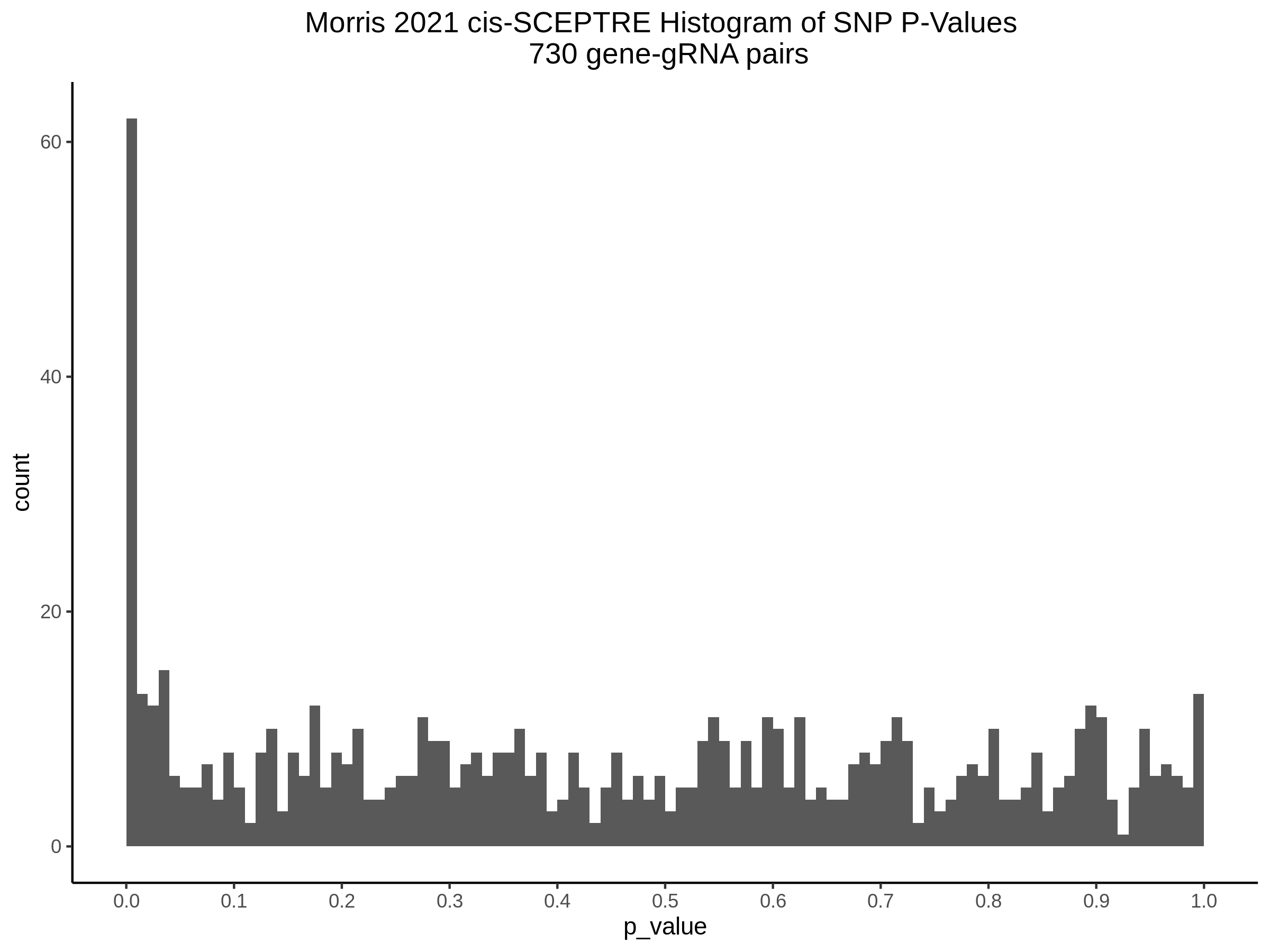
Morris 2021 cis-SCEPTRE All NTC gene-gRNA pair p values
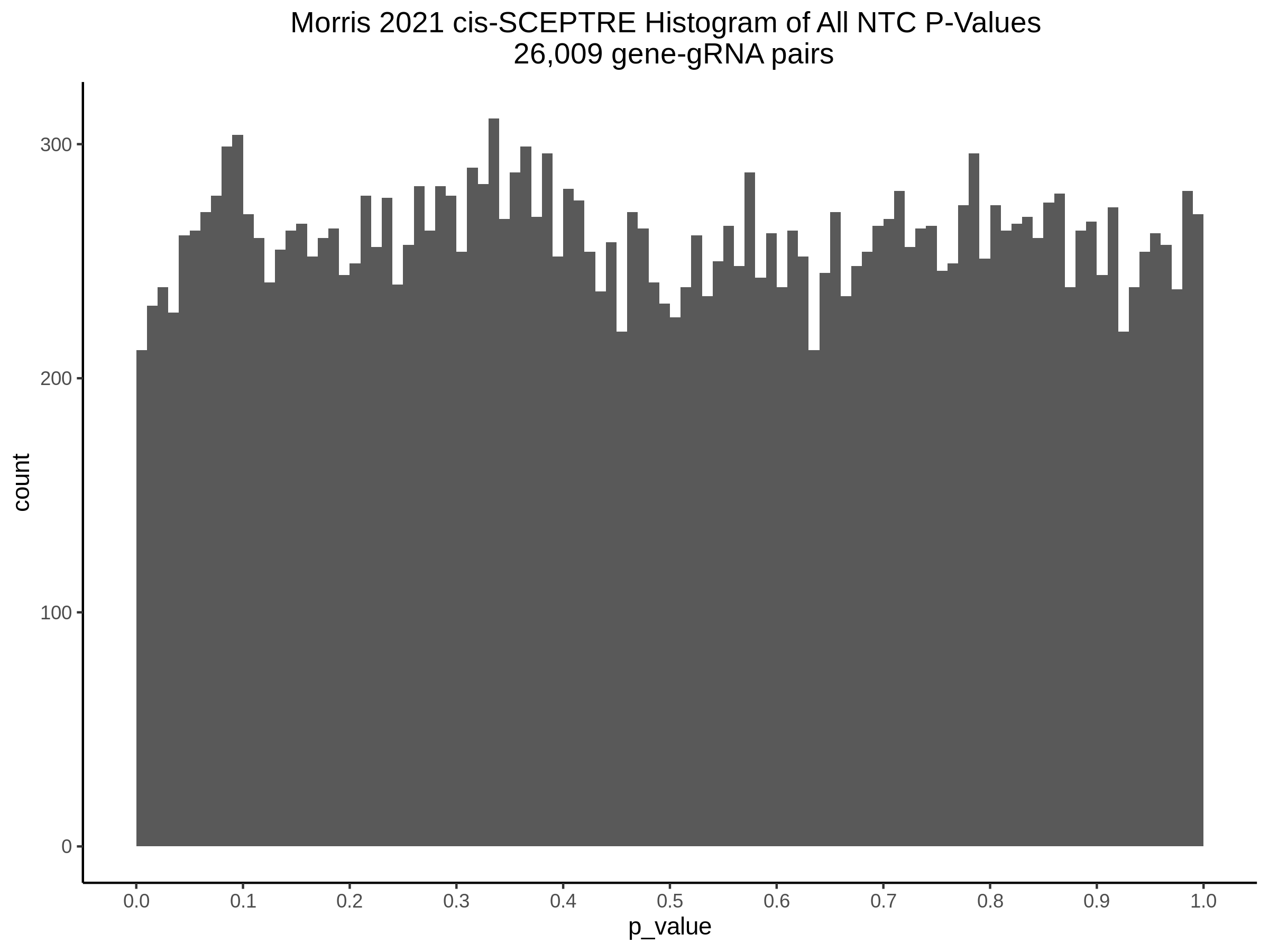
Histogram of P-Values in the Gasperini original cis-SCEPTE analysis: DHS, SNP, NTC.
Below are histograms of p-values for the original Gasp. cis analysis. Original is used to highlight analysis done by Morris on Gasp. data in the preprint. The preprint found 538 signals at FDR <=0.1, while our SCEPTRE run returned 586 signals at FDR <= 0.1.
Gasperini 2019 cis-SCEPTRE All DHS gene-gRNA pair p values
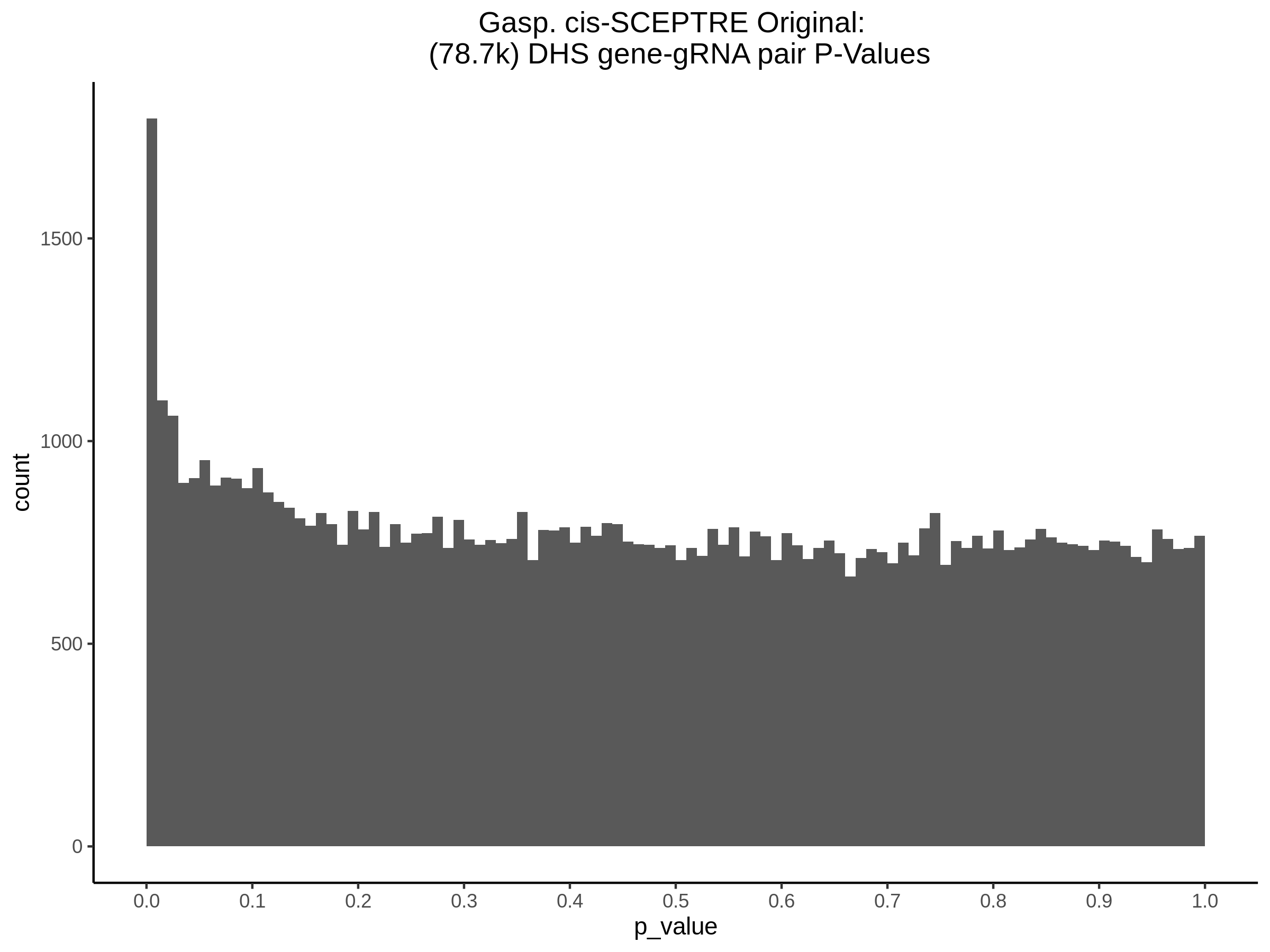
Gasperini 2019 cis-SCEPTRE All TSS gene-gRNA pair p values
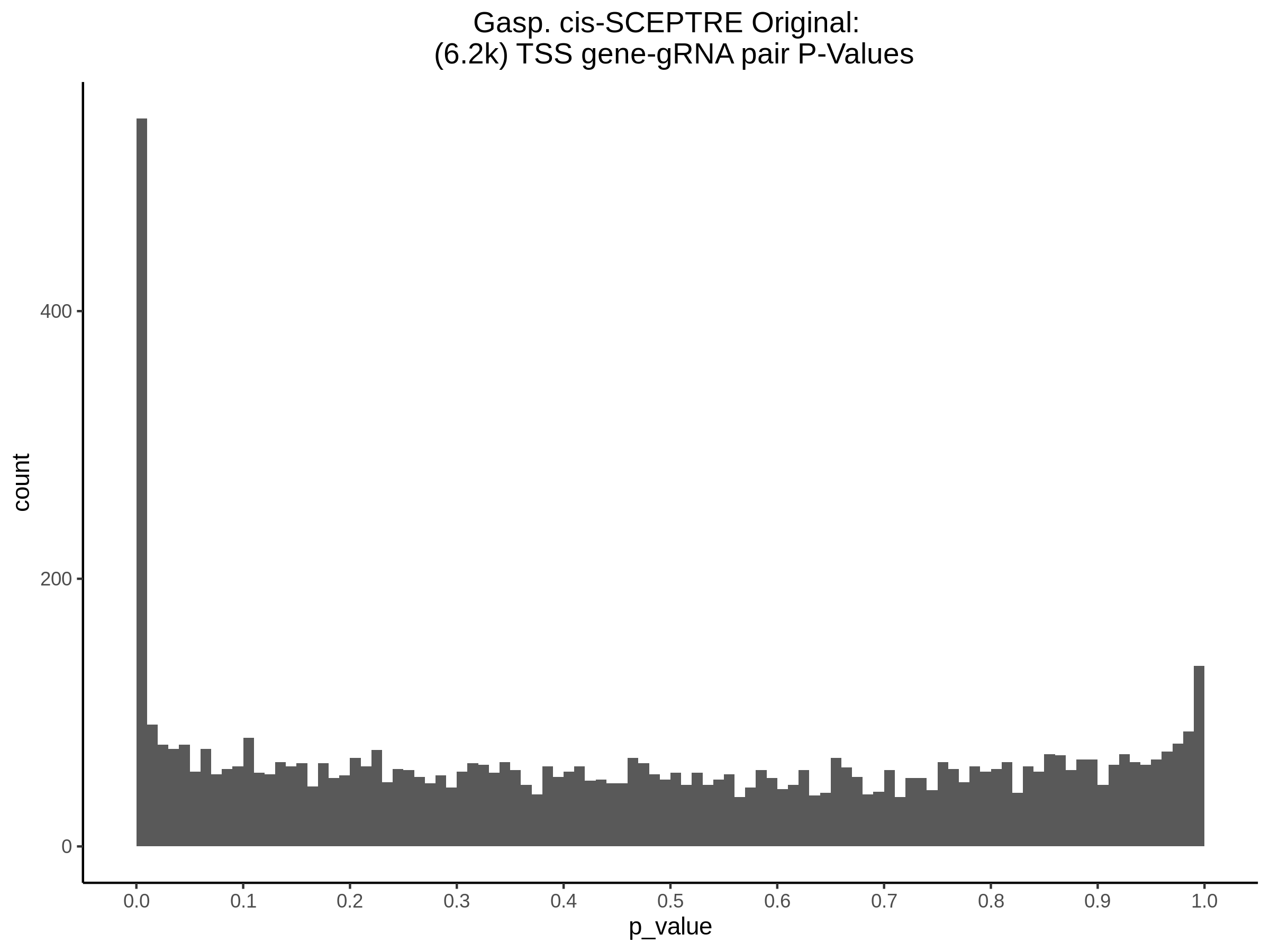
Gasperini 2019 cis-SCEPTRE All NTC gene-gRNA pair p values
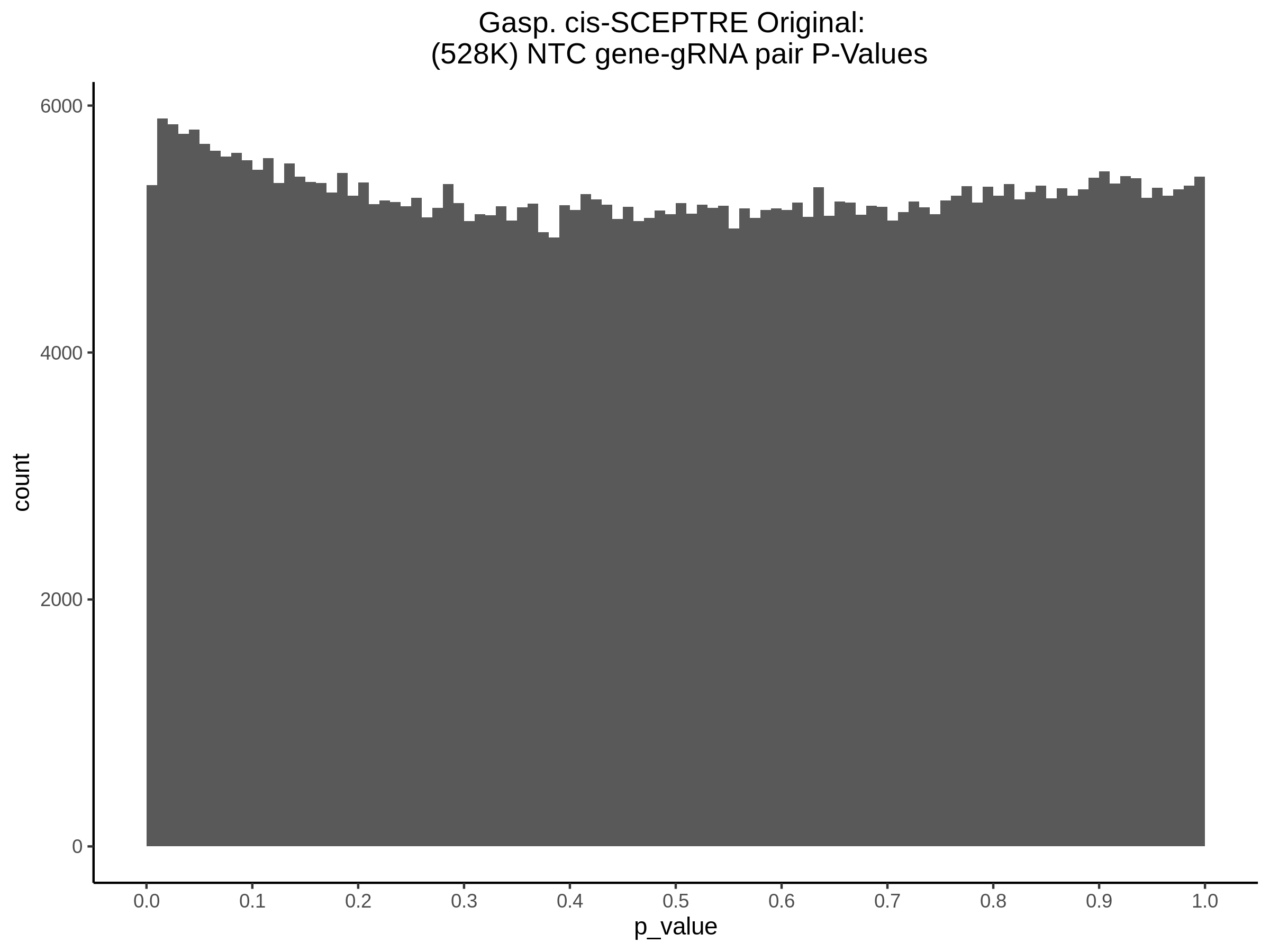
4/20/2022 Morris trans-wide SCEPTRE NTC QQPlots
Morris Transcriptome-wide NTC plotting
Statement of Problem: When running the original cis Morris analysis, NTC pairs were taken from the results reported in S3 of the Morris 2021 preprint. This resulted in 15.6k NTC gene-gRNA pairs. This plot is shown below for 3/23. Later, additional NTCs were spiked into the SCEPTRE, resulting in 26,009 total NTC pairs and plotted again on 4/13. See 4/13 for a table of gene-gRNA pairs run in cis.
During the transcriptome-wide SCEPTRE analysis of the Morris 2021 dataset, the NTC gRNAs were paired across all possible genes. See the first table in 4/18, which reports all gRNAs in the transcriptome-wide analysis for more information.
  r$> table(morris_trans_results %>% filter(site_type == 'NTC') %>% pull(gRNA_id))
  NTC-1 NTC-10 NTC-11 NTC-12  NTC-2  NTC-3  NTC-4  NTC-5  NTC-6  NTC-8  NTC-9
  10325  10325  10325  10325  10325  10325  10325  10325  10325  10325  10325
With NTCs, the general idea is to plot them in two ways, seperatly making the expected p values and together.
We make a qqplot for all the NTCs, setting our expected p value based on the aggregate of all the NTCs, and seperate them out into seperate plots (grid plots, cowplot).
# here we specifically make our neglog10_exp_pval based on ALL 113K NTCs (see table above, 11x10,325 pairs)
results_NTC_all = results_NTC_all %>% arrange(p_value) %>% mutate(quantile=1:nrow(results_NTC_all)/(nrow(results_NTC_all) + 1)) %>% mutate(neglog10_obs_pval = -log10(p_value), neglog10_exp_pval = -log10(quantile))![]()
Now, we make a qqplot for each individual NTCs, setting our expected p value based on that specific NTC, then plot.
  ntc9 = results %>% filter(gRNA_id == 'NTC-9')
  ntc9 = ntc9 %>% arrange(p_value) %>% mutate(quantile=1:nrow(ntc9)/(nrow(ntc9) + 1)) %>% mutate(neglog10_obs_pval = -log10(p_value), neglog10_exp_pval = -log10(quantile))
Expand NTC1
Expand NTC2
Expand NTC3
Expand NTC4
Expand NTC5
Expand NTC6
Expand NTC8
Expand NTC9
Expand NTC10
Expand NTC11
Expand NTC12
4/18/2022 Barplot/Table of Morris trans gene-gRNA pairs
The following is a barplot of gene-gRNA pairs run during the transcriptome wide analysis of Morris dataset. These include cis and trans pairs.
![]()
The following is a table of gene-gRNA pairs that are located trans to the target gRNA (>= 10Mb distance). The flag was made by checking the distance between gRNA and gene for each pair.
4/18/2022 Morris trans-wide SCEPTRE Analysis QQPlots
Below are qqplots for the Morris 2021 trans-wide analysis.
NTC QQPlot
Morris trans-wide NTC QQPlot
Matched NTC QQPlot
To generate this plot we selected the NTCs tested in the cis analysis below and took those pairs from the transcriptome-wide analysis of Morris 2021.
Morris trans-wide Matched-NTC QQPlot
SNP/PTC QQPlots
Morris trans-wide SNP QQPlot
Morris trans-wide PTC QQPlot
Morris trans-wide QQPlot
Morris trans-pairs P-value histogram
Morris trans-wide P-value histogram
4/13/2022 Morris cis-SCEPTRE Analysis QQPlots w/ Additional NTCs
Morris 2021 cis gene-gRNA pair results w/ additional NTCs
This builds upon the results reported below on 3/23 by including additional NTCs.
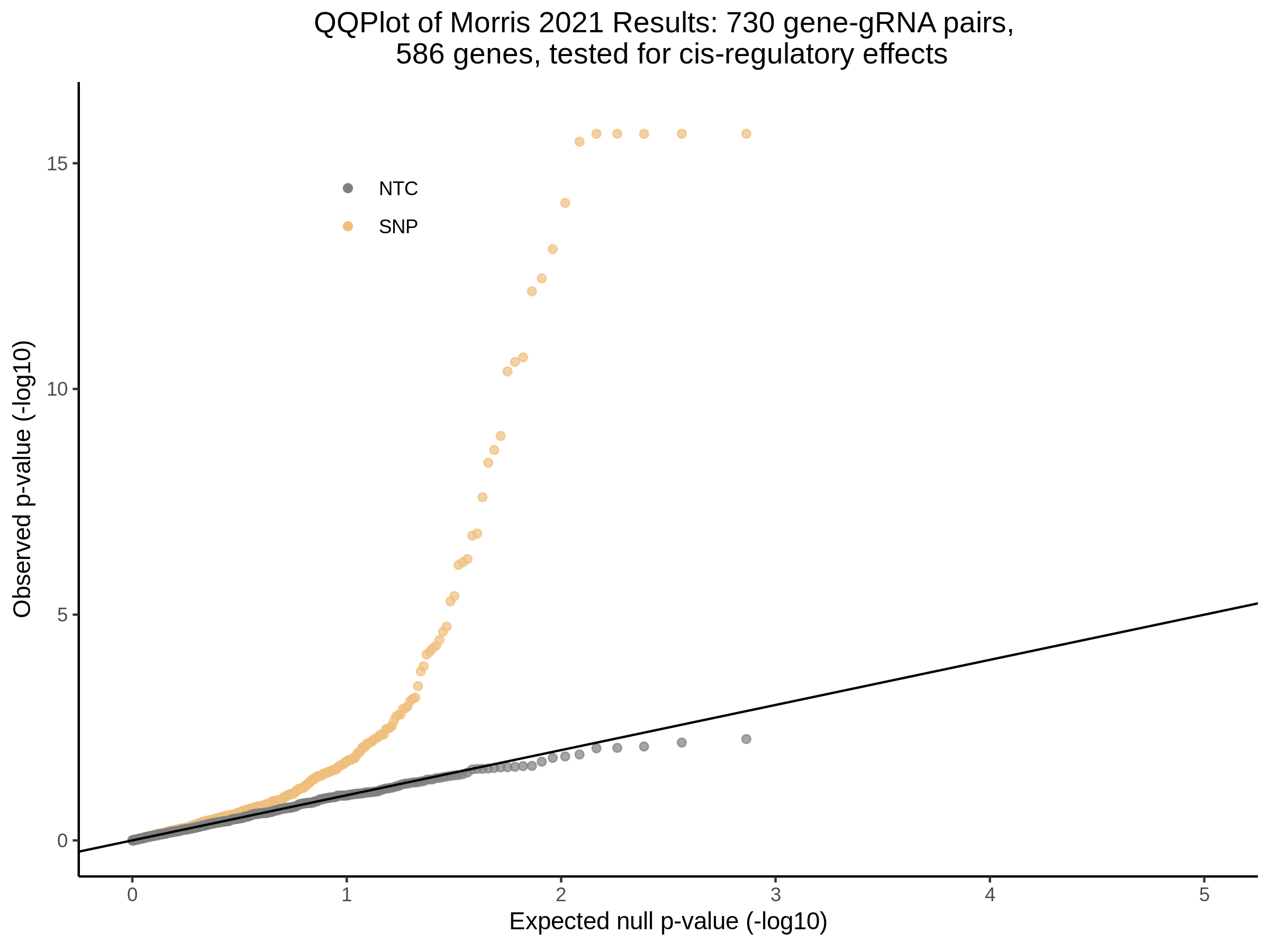
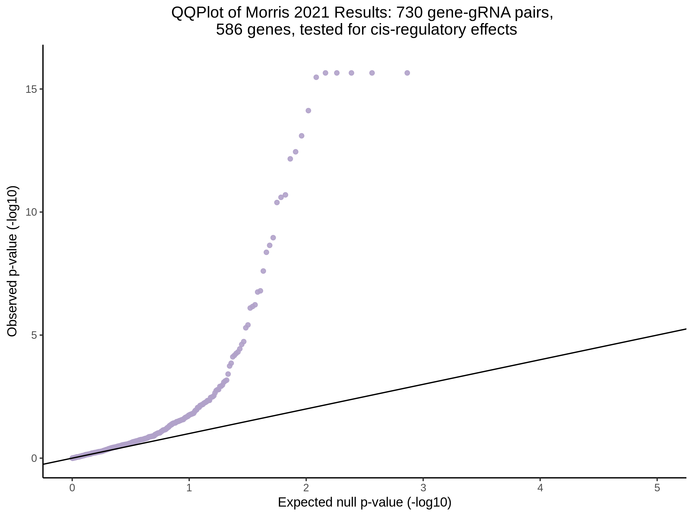
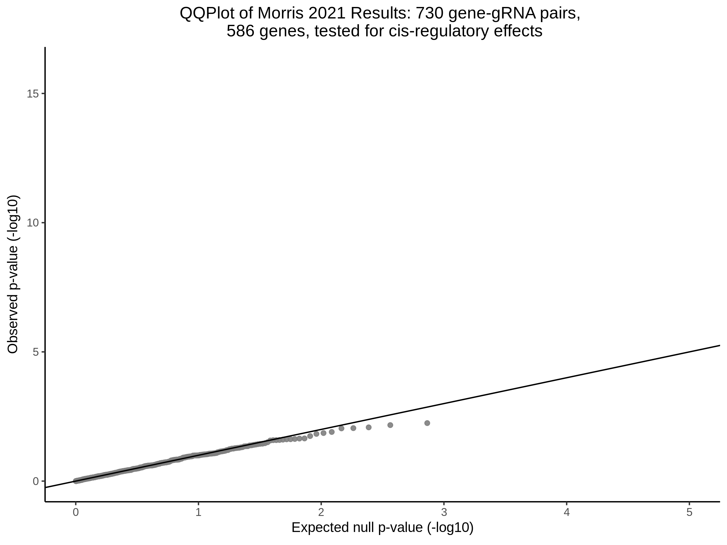
All NTCs (26,009 pairs):
In order to add additional NTCs, I spiked in extra by assigning my favorite NTCs to all availible genes in the dataset (10325). This results in a new amount of NTCs: 26,009.
 NTC-1 NTC-10 NTC-11 NTC-12  NTC-2  NTC-3  NTC-4  NTC-5  NTC-6  NTC-7  NTC-8  NTC-9
   475  10325    456    536    579    601    511    523    583  10325    578    517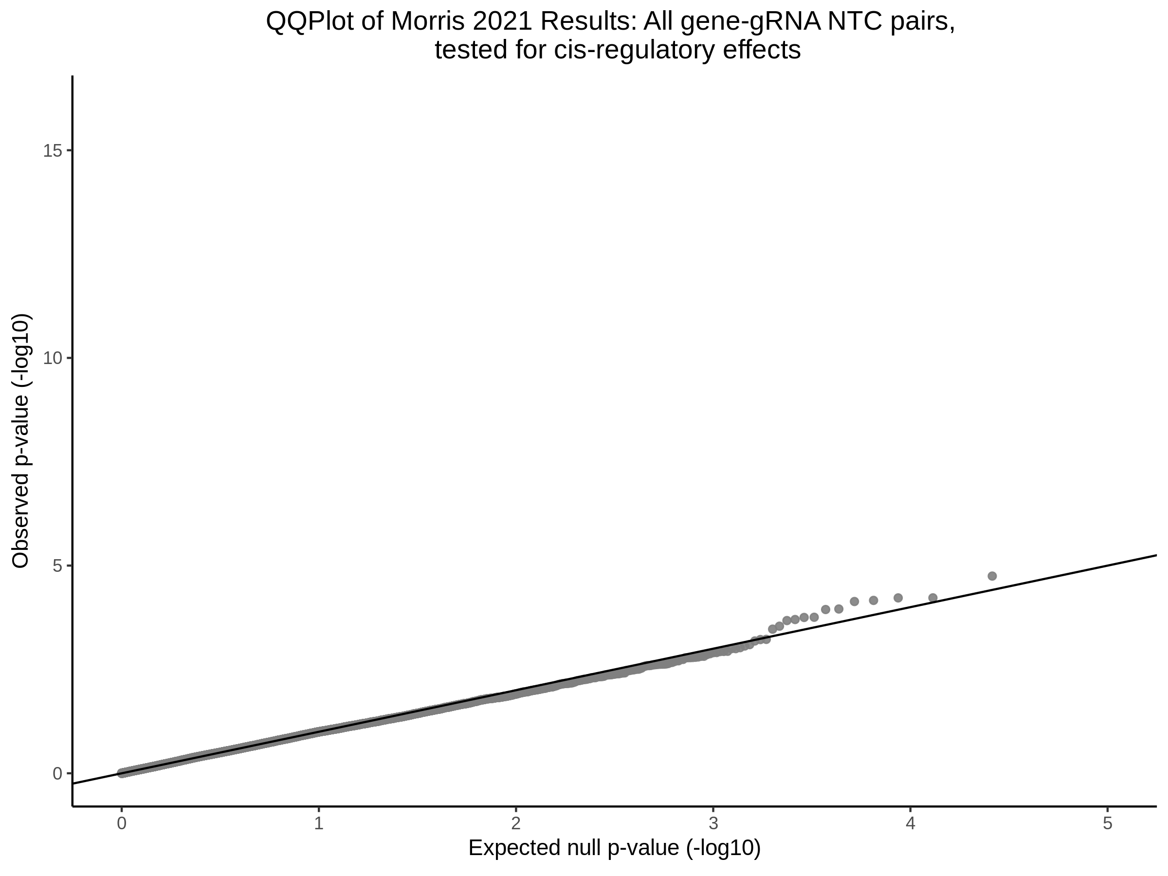
Histogram:
3/30/2022 Morris trans-wide Matched NTC QQPlot
The is the trans portion of the preprint: defined as trans-effects upon cCRE perturbation. Notes on preparing the trans-pairs for this analysis:
- The gene gRNA pairs were not prepared exactly correctly (as was done for the super massive Gasperini dataset)
- Pairs were prepared by iterating through all availible gRNAs in the
QCed dataset (185) and matching them to all possible genes (10325) in
the dataset.
- This ignored the possibility of creating cis pairs and results in testing all possible pairs in the dataset (1.7M).
- A more correct approach was later written for the trans pairs in the Gasperini dataset where location info is taken into account in order to define trans pairs as > 10 Mb distance on the same chromosome or different chromosome.
- An example of the code used for the Morris trans pairs below:
gRNA_gene_pairs_SCEPTRE = data.table()
for (gRNA in ondisc_gRNAs){
    df = data.table(gene_id = ondisc_genes) %>% mutate(gRNA_id = gRNA)
    gRNA_gene_pairs_SCEPTRE = rbindlist(list(gRNA_gene_pairs_SCEPTRE, df))
}
Morris trans-wide SCEPTRE Matched NTCs (15.6k NTC)
These NTCs were originally tested in the cis results (see 3/23/2022 below). To generate this plot we selected the NTCs tested in the cis analysis below and took those pairs from the transcriptome-wide analysis of Morris 2021. In other words, this plot does not include all NTCs tested in the trans analysis of Morris 2021 data.
![]()
3/23/2022 Morris cis-SCEPTRE Analysis QQPlots
Morris 2021 Results for cis gene-gRNA pairs
The is the cis portion of the preprint: defined as cis-effects upon cCRE perturbation. There are 730 gene gRNA pairs that correspond to the SNP targeting results, while there are 15.6k NTC gene-gRNA pairs. For the combined plot, non-targeting gRNA-to-gene pairs were randomly sampled from the same set of genes tested in cis for targeting gRNAs.
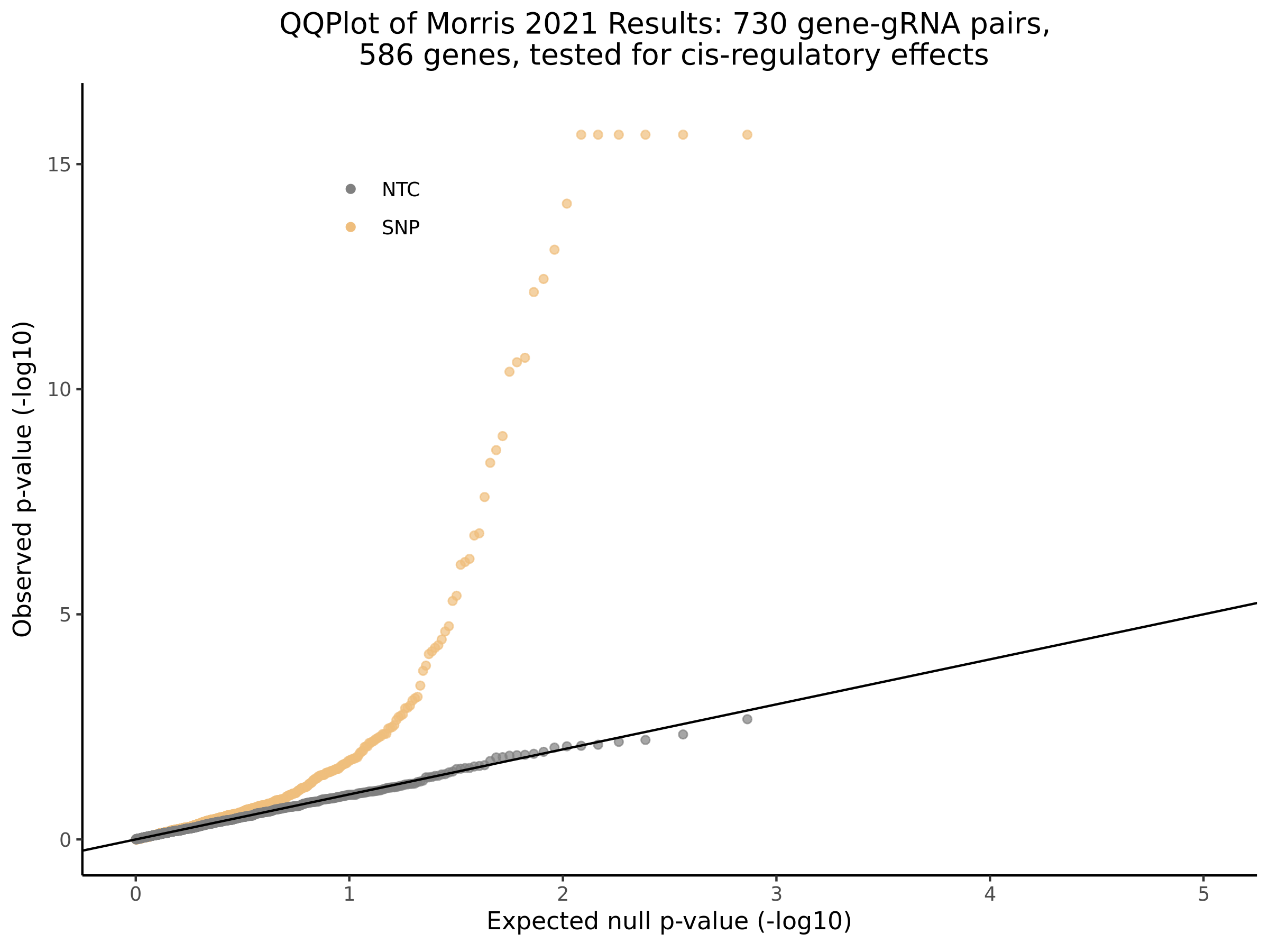
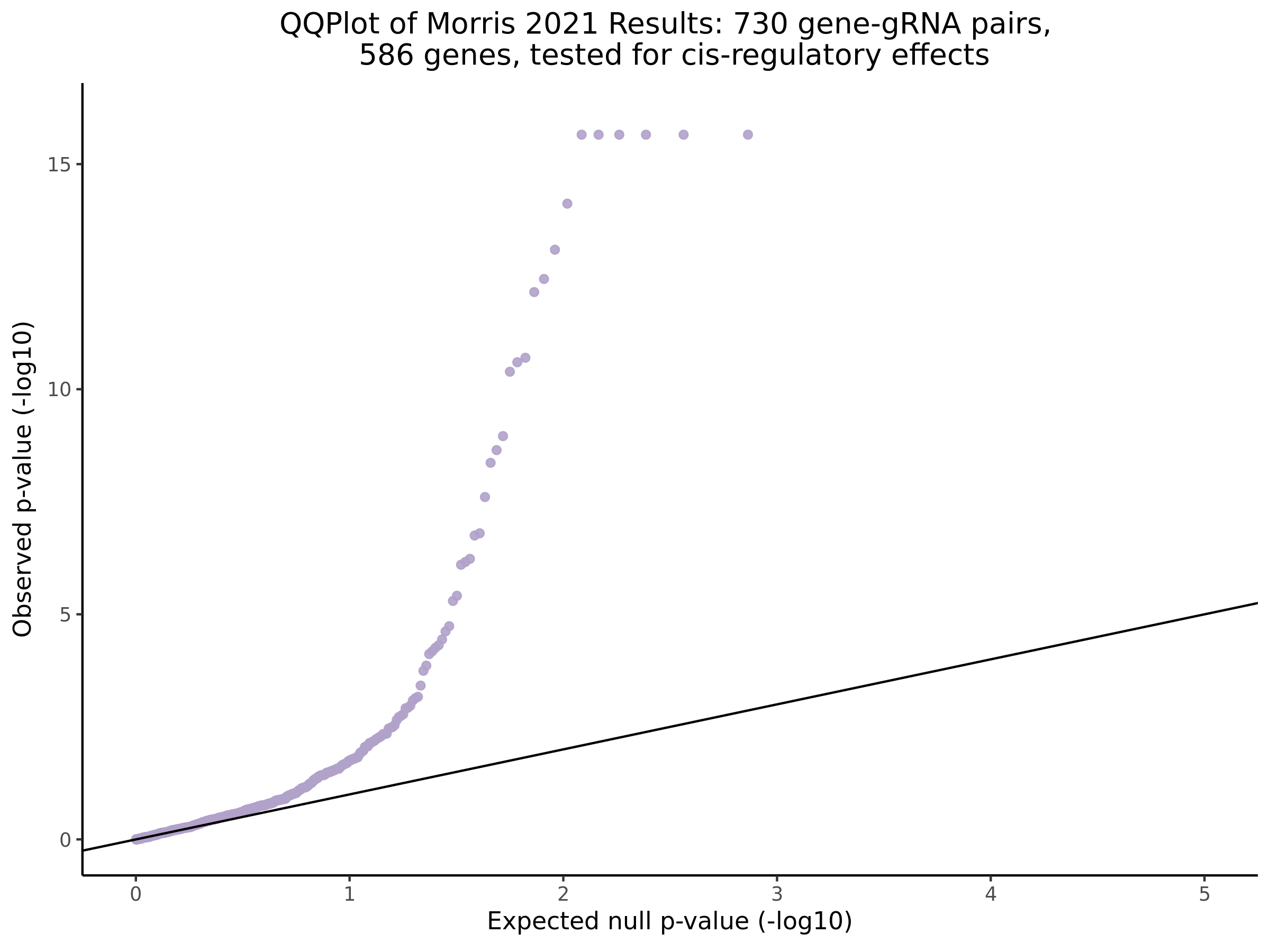
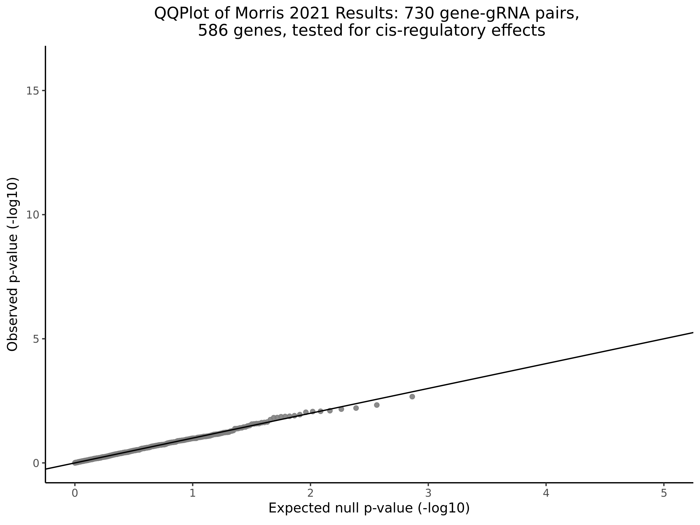
All NTCs (15.6k):
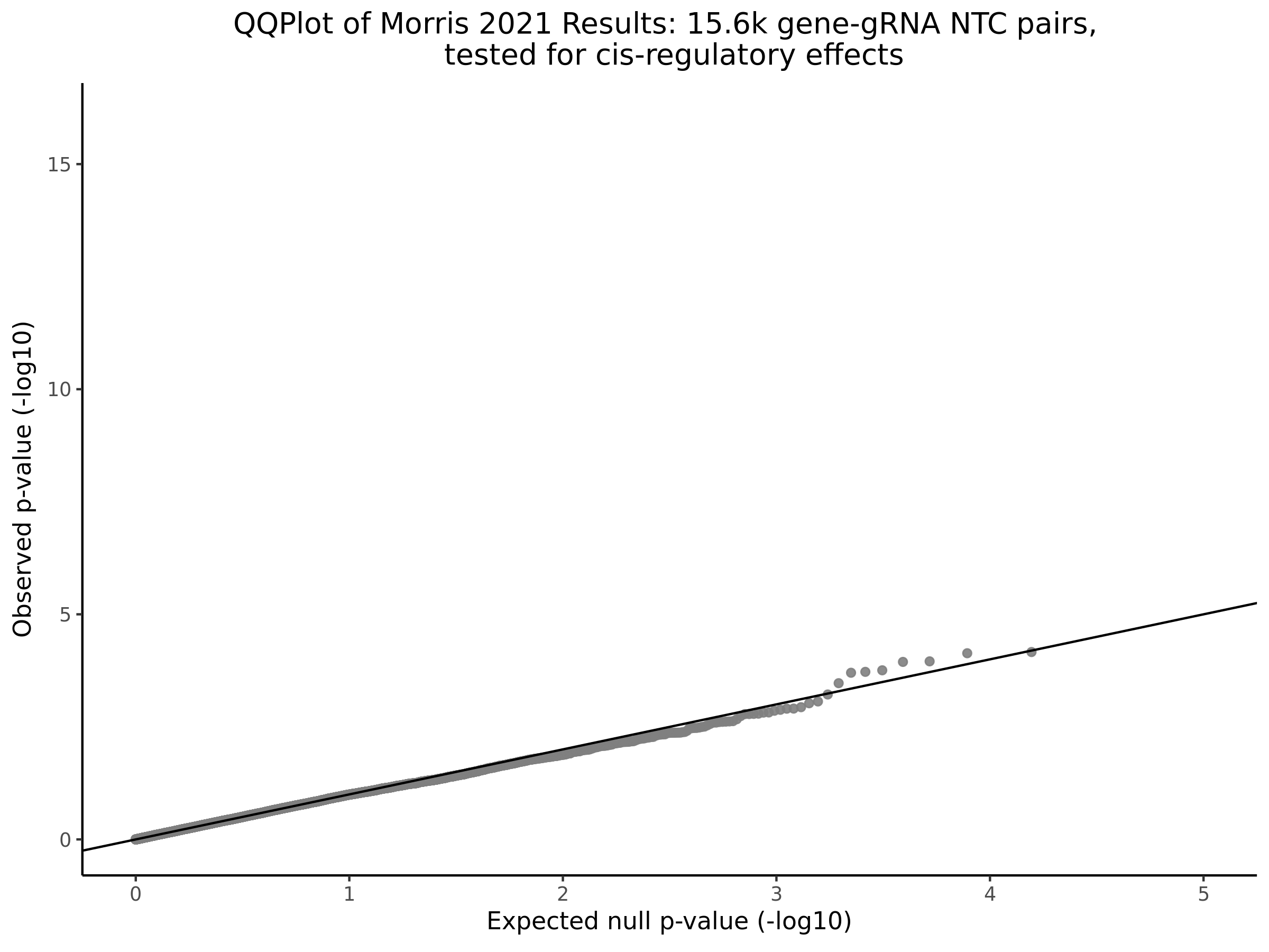
Notes on preparing Gasperini trans-wide analysis
The goal here is to prepare a set of gene gRNA pairs to be used for testing for trans gene regulation within the Gasperini 2019 dataset.
- There are 5,723 enhancer targetting gRNAs in the Gasperini 2019 dataset
- Off the bat the main consideration is that the Gasperini dataset
uses ensembl IDs + b37 reference.
- To get the b37 ref genome:
library(biomaRt) library(dplyr) #grch37 = useEnsembl(biomart="ensembl",GRCh=37) #listDatasets(grch37) # what is availible rn (the last release aka 37.p13) ensembl = useEnsembl(biomart="ensembl", dataset="hsapiens_gene_ensembl", GRCh=37) listAttributes(ensembl) # list what attributes we can pull ie: gene, chromosome, position, etc b37_reference <- getBM(attributes=c('ensembl_gene_id','ensembl_transcript_id','hgnc_symbol', 'gene_biotype', 'strand', 'chromosome_name','start_position','end_position', 'entrezgene_id','description'), mart = ensembl) - Create the actual pairs with these rules:
- Gene must be >= 10 Mb from targetted DHS enhancer
- OR Gene is on other chromosome
- Make sure to use registerDoParallel because rbinding 76M pairs will
take a while on 1 core
- Notice the custom combine function and multicombine set to TRUE (allowing custom combine to take more that 2 args).
# original_results_raw <- suppressWarnings(read_tsv(paste0('/project2/xuanyao/nikita/SCEPTRE/data_matrixes/Gasperini_2019_dataset/at_scale_data/GSE120861_all_deg_results.at_scale.txt'), col_types = 'cddddddccccciiciiccl'))
# dhs_enhancer_pairs = original_results %>% filter(site_type == "DHS" & quality_rank_grna == "top_two") %>% select(gene_id, site_type, grna_group, target_site, target_site.start, target_site.stop, chr) %>% distinct(grna_group, .keep_all = TRUE)
# Notice that dhs_enhancer_pairs is a selection of results for DHS + top two AND we perform distinct(grna_group) to isolate unique gRNAs to make the pairs from.
dhs_enhancer_pairs = as_tibble(data.table::fread(paste0('/home/nbabushkin/stingseq_scripts/Gasperini_78kDHS_pairs_table.csv'), stringsAsFactors = F, header = T, sep=','))
tss_pairs = as_tibble(data.table::fread(paste0('/home/nbabushkin/stingseq_scripts/Gasperini_6kTSS_pairs_table.csv'), stringsAsFactors = F, header = T, sep=','))
approved_chrs = paste0('chr', seq(1,22))
library(GenomicRanges)
annotated_genes = annotations %>% select(hgnc_symbol, chromosome_name, start_position, end_position, ensembl_gene_id) %>% filter(ensembl_gene_id %in% approved_genes) %>% mutate(chromosome_name = paste0('chr', chromosome_name))
annotated_genes = annotated_genes %>% distinct(hgnc_symbol, chromosome_name, start_position, end_position, ensembl_gene_id)
colnames(annotated_genes) <- c("GeneSymbol","Chr","Start","End",'ensembl_gene_id')
annotated_genes
genes_GR <- makeGRangesFromDataFrame(annotated_genes,keep.extra.columns = TRUE)
genes_GR <- keepStandardChromosomes(genes_GR, pruning.mode="coarse")
print(paste0('starting tss_pairs loops...'))
tic()
df1 = foreach (x=1:nrow(tss_pairs),
              .combine=function(...) rbindlist(list(...)),
              .multicombine=TRUE) %dopar% {
                gRNA = tss_pairs[x, 'grna_group'] %>% pull()
                s = tss_pairs[x, 'target_site.start'] %>% pull()
                e = tss_pairs[x, 'target_site.stop'] %>% pull()
                c = tss_pairs[x, 'chr'] %>% pull()

                query <- GRanges(c, IRanges(ifelse(s > 1e7, s - 1e7, 1), e + 1e7, id = gRNA))
                genes_on_chr = annotated_genes %>% filter(Chr == c) %>% pull(ensembl_gene_id) %>% unique()
                genes_not_on_chr = annotated_genes %>% filter(Chr %in% approved_chrs & Chr != c) %>% pull(ensembl_gene_id) %>% unique()
                #f = findOverlaps(query, genes_GR, ignore.strand=TRUE)
                inrange = genes_GR[overlapsAny(genes_GR, query[1])]
                inrange_genes = inrange$ensembl_gene_id %>% unique()
                out_of_range_genes = setdiff(genes_on_chr, inrange_genes)

                genes = c(out_of_range_genes, genes_not_on_chr) %>% unique()
                #cat(paste0(gRNA ,' :: # genes found: ', length(genes), ' \n'))
                df = data.table(gene_id = genes) %>% mutate(gRNA_id = gRNA)
                # if (x %% 100 == 0){cat(paste0('status: ', x, '/', nrow(tss_pairs), ' - ',Sys.time(),' \n'))}
                return(df)
}
toc()
print(paste0('starting dhs_enhancer_pairs loops... '))
tic()
df2 = foreach (x=1:nrow(dhs_enhancer_pairs),
              .combine=function(...) rbindlist(list(...)),
              .multicombine=TRUE) %dopar% {
                gRNA = dhs_enhancer_pairs[x, 'grna_group'] %>% pull()
                s = dhs_enhancer_pairs[x, 'target_site.start'] %>% pull()
                e = dhs_enhancer_pairs[x, 'target_site.stop'] %>% pull()
                c = dhs_enhancer_pairs[x, 'chr'] %>% pull()

                query <- GRanges(c, IRanges(ifelse(s > 1e7, s - 1e7, 1), e + 1e7, id = gRNA))
                genes_on_chr = annotated_genes %>% filter(Chr == c) %>% pull(ensembl_gene_id) %>% unique()
                genes_not_on_chr = annotated_genes %>% filter(Chr %in% approved_chrs & Chr != c) %>% pull(ensembl_gene_id) %>% unique()
                #f = findOverlaps(query, genes_GR, ignore.strand=TRUE)
                inrange = genes_GR[overlapsAny(genes_GR, query[1])]
                inrange_genes = inrange$ensembl_gene_id %>% unique()
                out_of_range_genes = setdiff(genes_on_chr, inrange_genes)

                genes = c(out_of_range_genes, genes_not_on_chr) %>% unique()
                #cat(paste0(gRNA ,' :: # genes found: ', length(genes), ' \n'))
                df = data.table(gene_id = genes) %>% mutate(gRNA_id = gRNA)
                #if (x %% 100 == 0){cat(paste0('status: ', x, '/', nrow(dhs_enhancer_pairs), ' - ',Sys.time(),' \n'))}
                return(df)
}
toc()
gRNA_gene_pairs_SCEPTRE = rbindlist(list(df1, df2)) # used in the %dopar%  above, as well
# final cleaning/sanity function
gRNA_gene_pairs_SCEPTRE = gRNA_gene_pairs_SCEPTRE %>% filter(gRNA_id %in% onidsc_gRNAs, gene_id %in% ondisc_genes)
Note: make sure to set up registerDoParallel(cores=XX) correctly prior otherwise it will take >1hr to bind the 76M pairs together.
3/7/2022
Morris 2021 Data Processing Notes
Notes on preparing SCEPTRE for Morris 2021 data:
Single Cell Data Processing within STINGseq:
- Matrixes prepared in kallisto|bustools scRNA seq pipeline
- Seurat v3.0.0 was used to work matrixes
cDNA/GDO matrixs processing:
- filter: cells <= 20% mito reads + cells >= 850 unique gene UMI
- resulting matrix: 14,775 cbcs + 3875 median genes per cell
#   cDNA QC FILTER
sobject_expression_subset <- subset(sobject_expression, subset = nFeature_RNA >= 850 & percent_mito < 20, cells = common_cellbarcodes)
# 35606 features across 14813 samples within 1 assay
# this is 28 cells OFF from the manuscript
median_genes_per_cell = median(sobject_expression_subset@meta.data$nFeature_RNA)
# result: 3899
# paper: 3875
cDNA_cells = colnames(sobject_expression_subset) # get the cells that passed expression QC above
HTO matrix:
- HTO QC: at least one HTO detected per cell and less than 2,500 total
HTO UMIs per cell.
- We center-log-ratio (CLR) transformed the HTO UMI counts and demultiplexed cells by their transformed HTO counts to identify singlets.
- threshold of 0.91 maximized the number of singlets detected to 9,520 while reducing the number of multiplets (multiple cells per droplet) to 2,482 and empty cells to 2,726.
GDO matrix:
- We used the 9,520 singlets to then process the gRNA (GDO) UMI count matrix, identifying 9,507 cells after removing cells with more than 15,000 total GDO UMIs.
- We observed that a minimum of 5 UMIs per gRNA resulted in a stable
threshold as the number of cells per gRNA does not change with higher
thresholds
- This is a reference to the threshold use to define the logical GDO or gRNA matrix within ondisc preprocessing
sobject_expression_subset <- NormalizeData(sobject_expression_subset, normalization.method = 'CLR') # normalize data w/ CLR transform
# "We used the HTODemux function and determined a threshold of 0.91 maximized the number of
#   singlets detected to 9,520 while reducing the number of multiplets (multiple cells per droplet) to
#   2,482 and empty cells to 2,726."
sobject_expression_subset <- HTODemux(sobject_expression_subset, assay = 'HTO', positive.quantile = 0.91)
2/28/2022
SCEPTRE Gasperini 2019 Downsampling Results
These are the results on 78k DHS enhancers in Gasperini 2019 across multiple conditions.
Effect of Cell Count
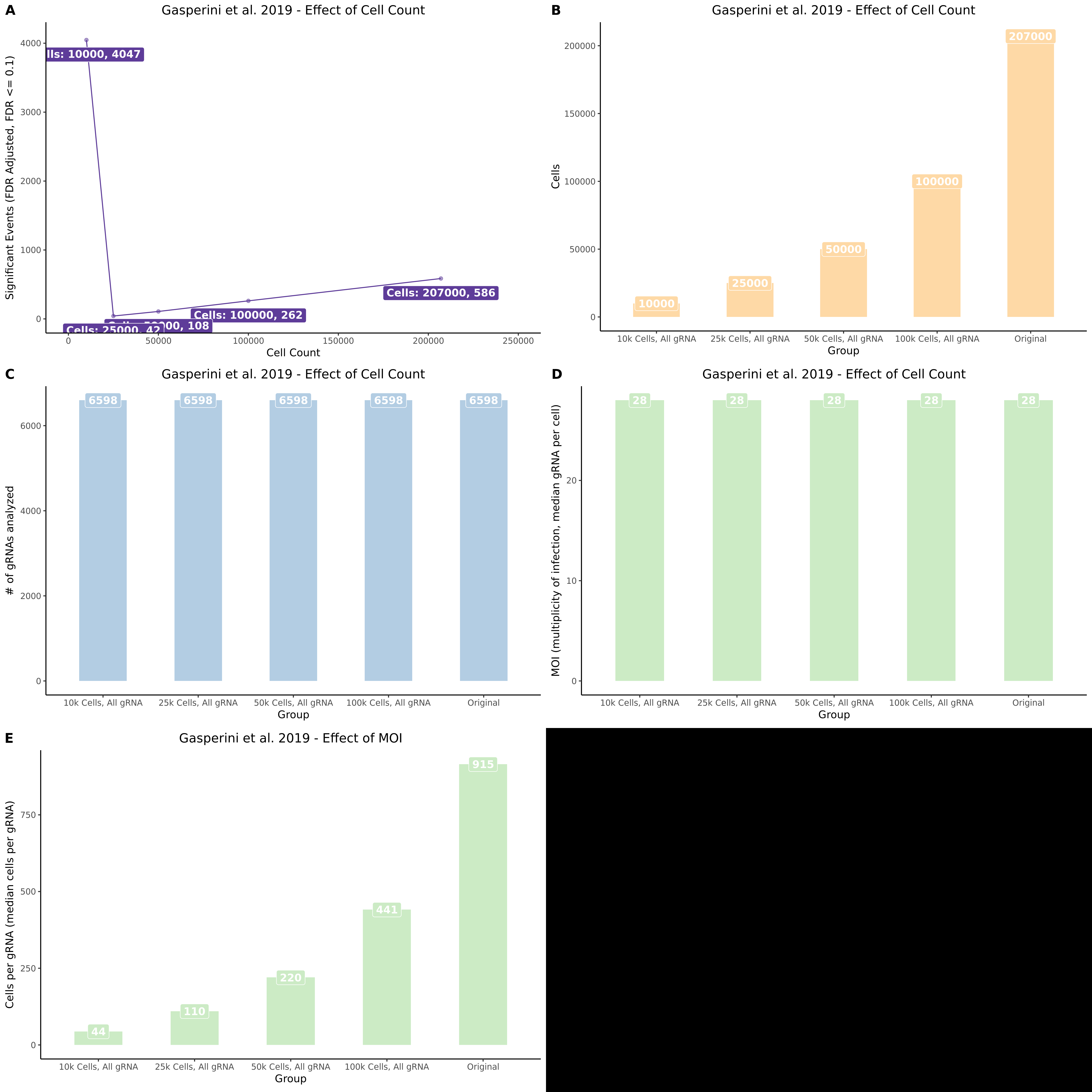
Effect of gRNA pairs
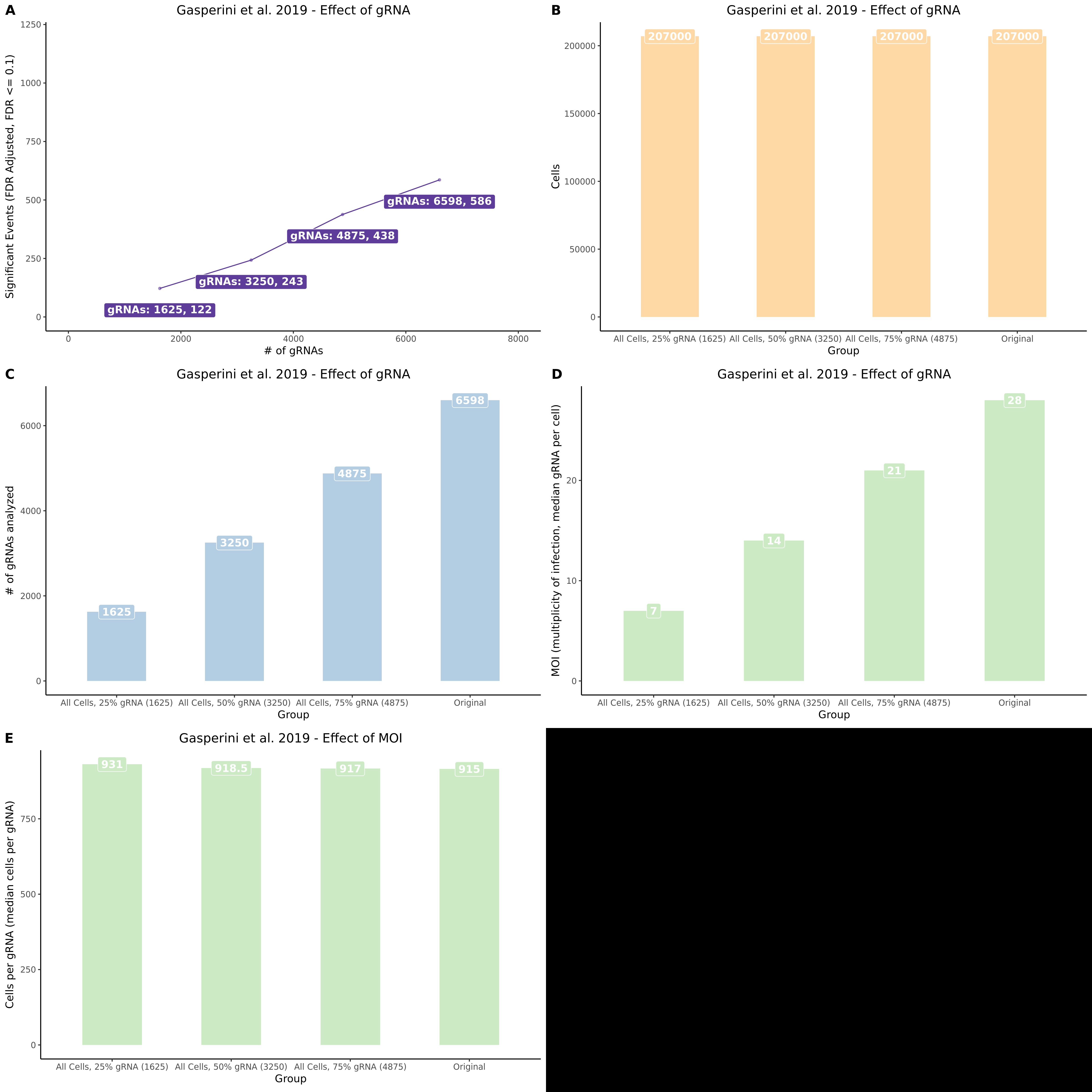
Effect of MOI
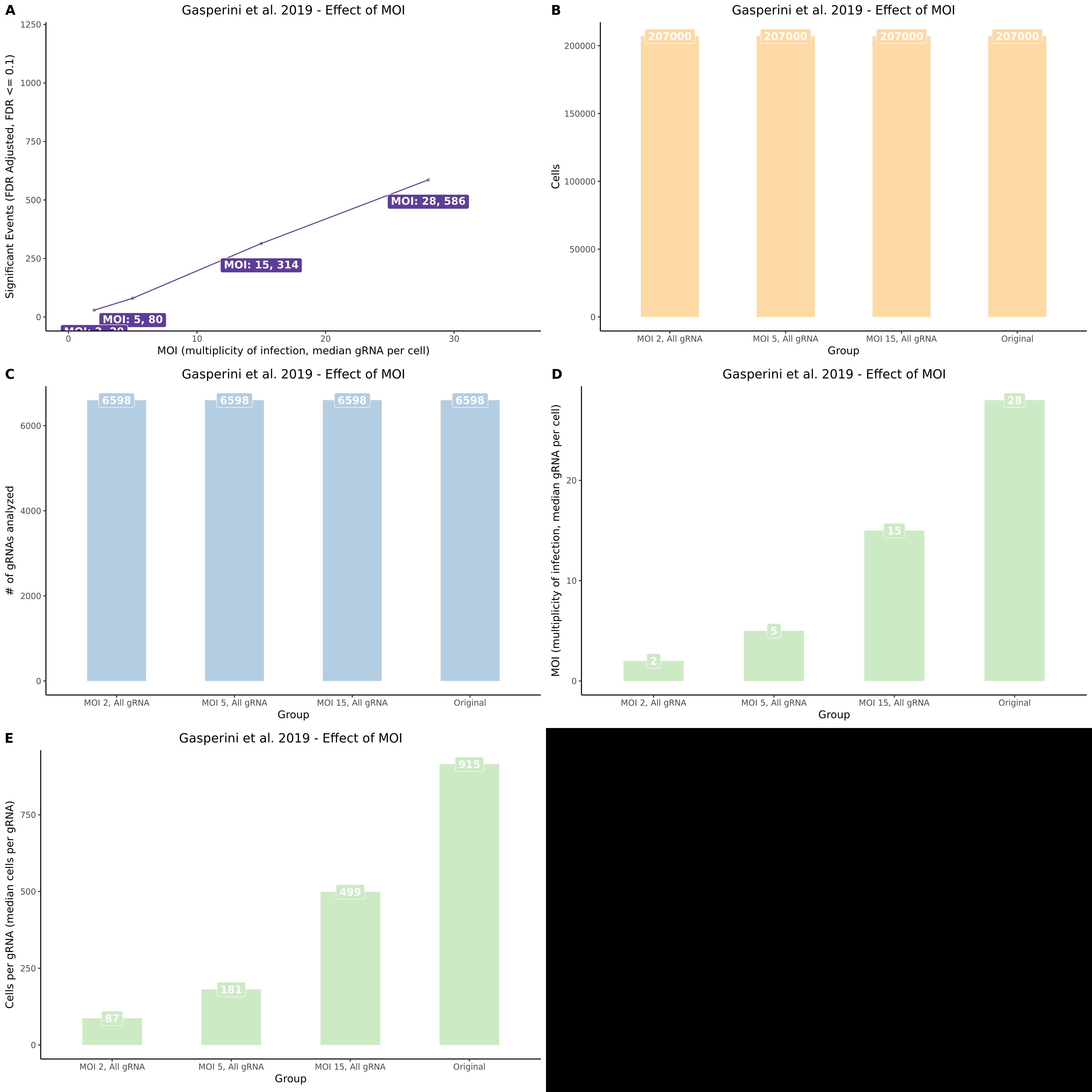
Zscore vs TSS distance / TSS distance Distribution
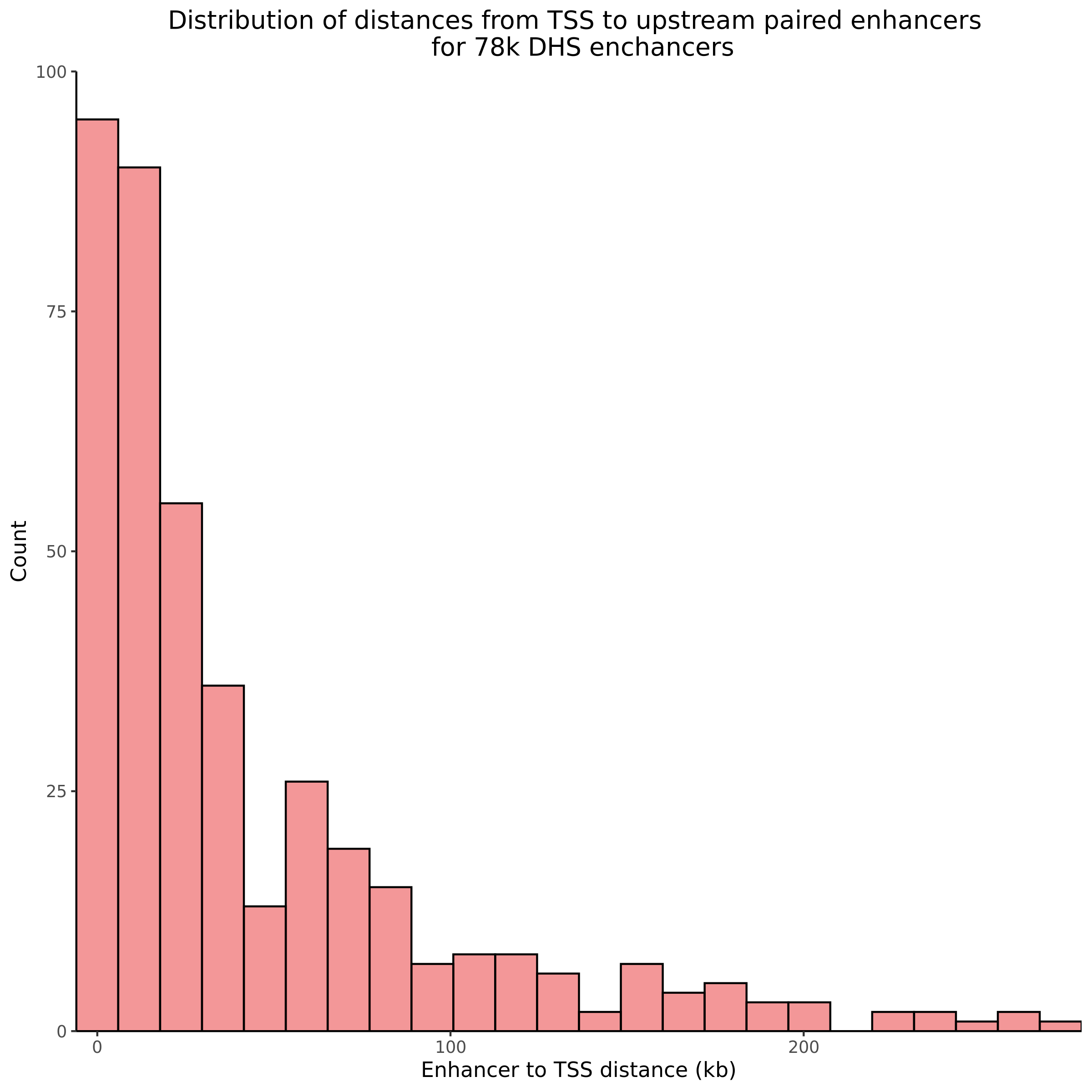
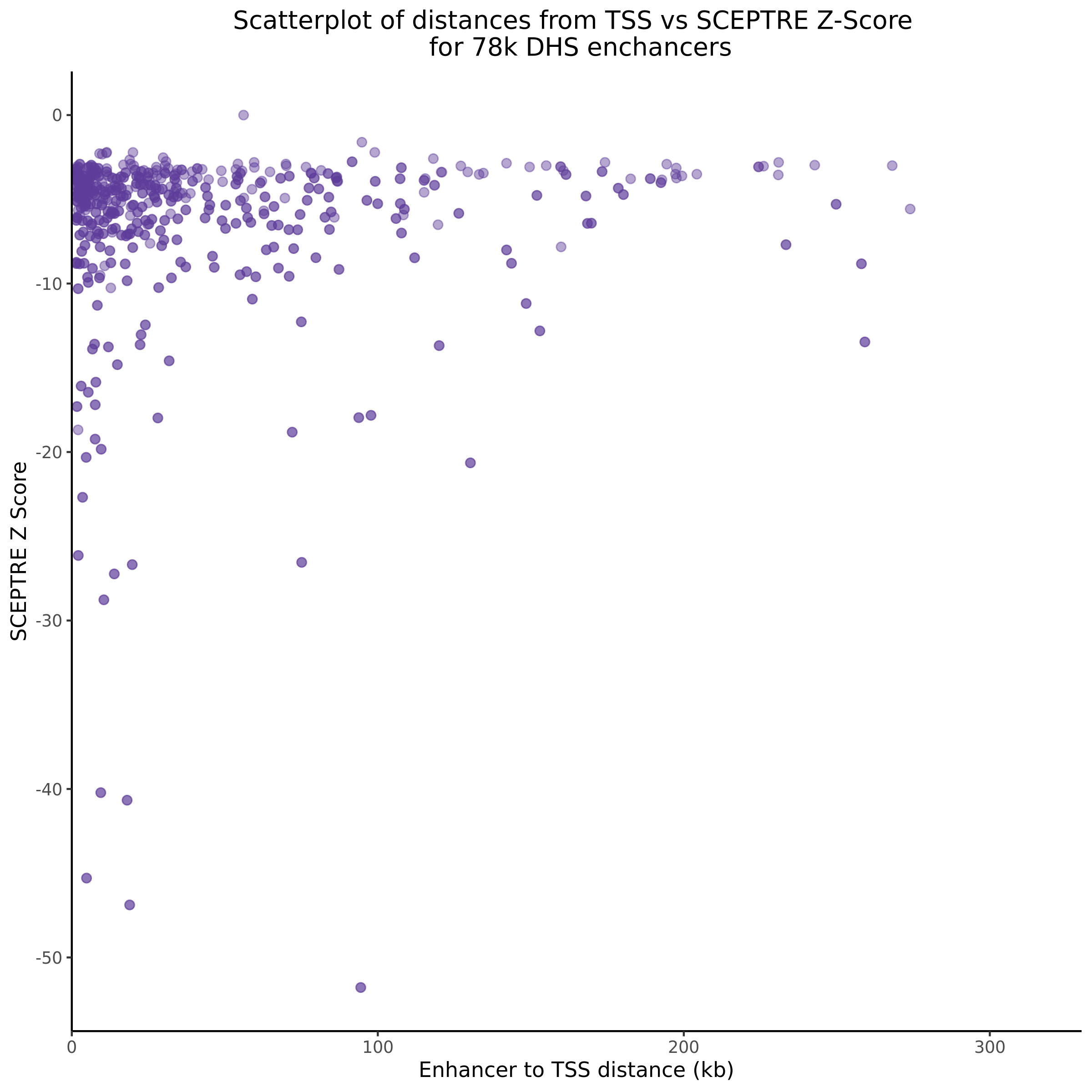
Comparing the SCEPTRE results:
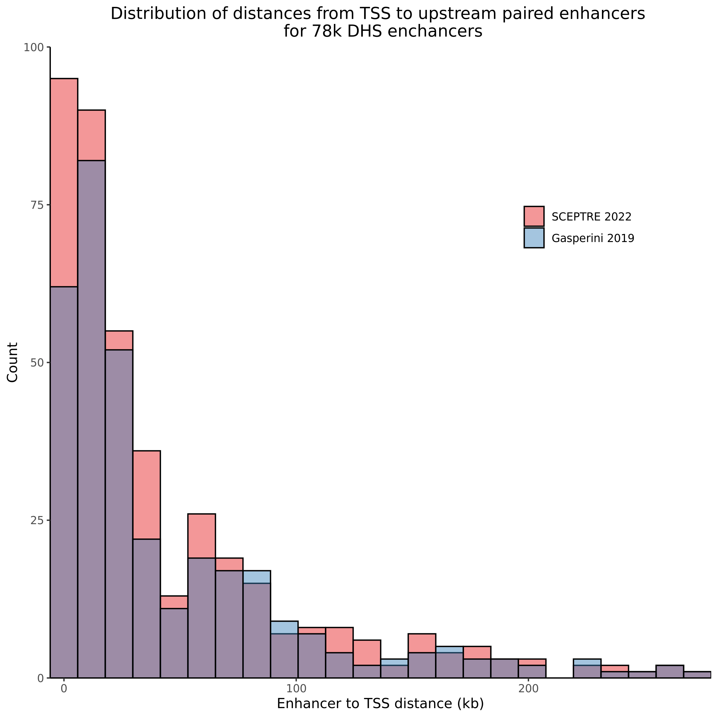
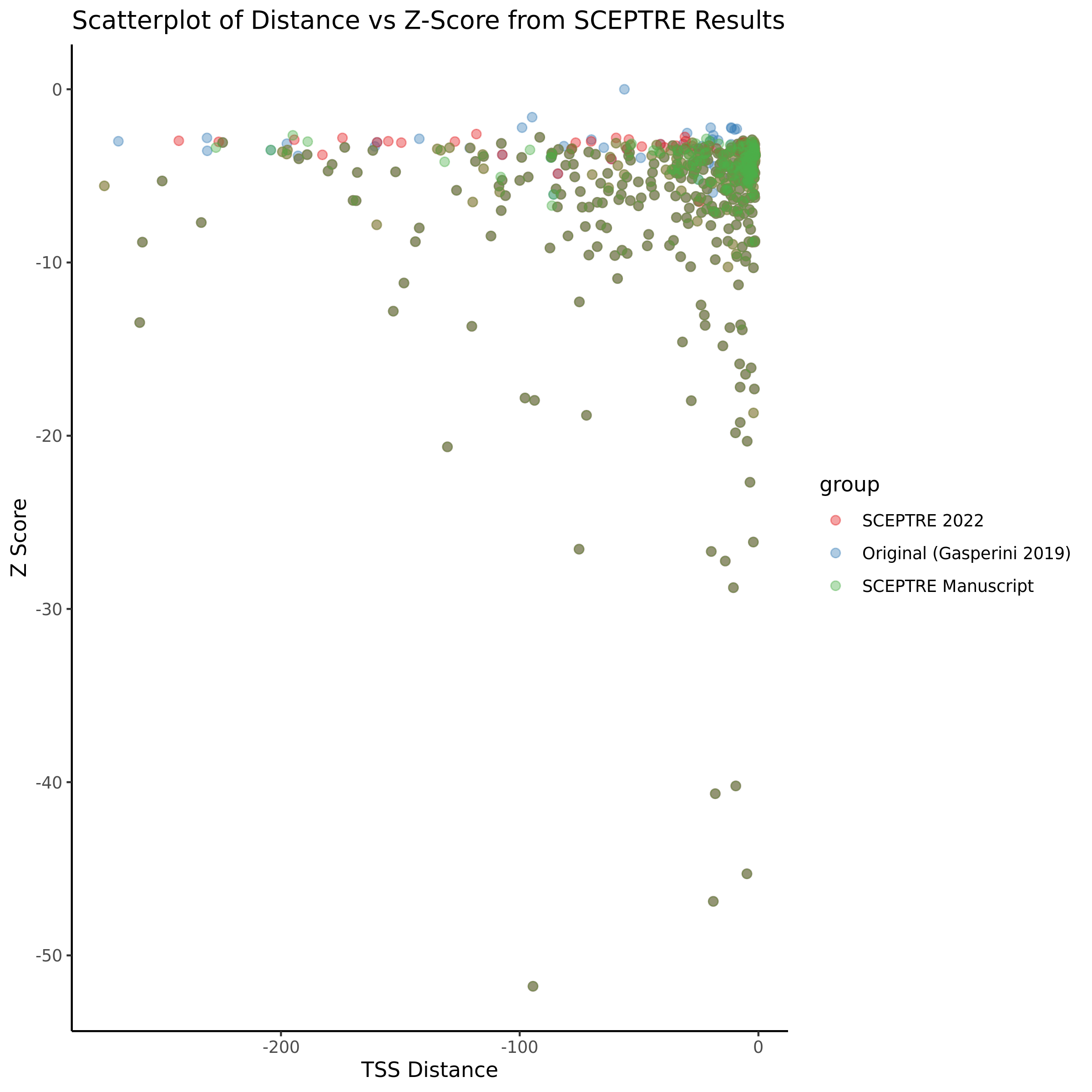
2/7/2022
SCEPTRE Downsampling QC Results
The goal was to downsample and evaluate SCEPTRE performance on NTCs/SNPs across downsampled MOI, cell count, and gRNAs in Gasperini 2019. The plots below show some of the QC results from the downsampled datasets prior to running SCEPTRE.
All Cells 10kgRNAs


100k Cells (~50%) 10kgRNAs

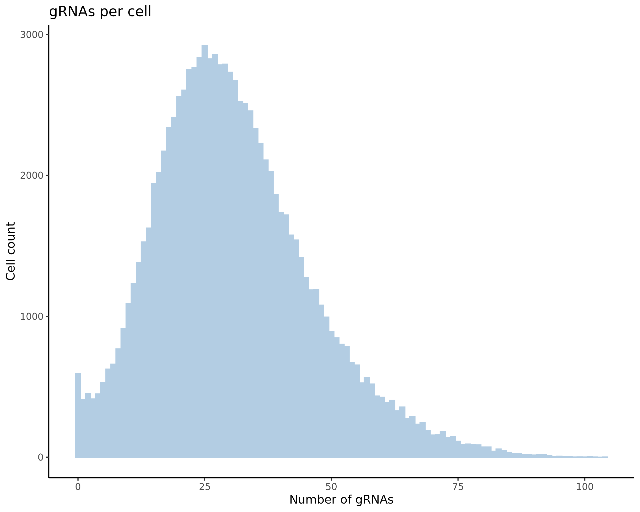
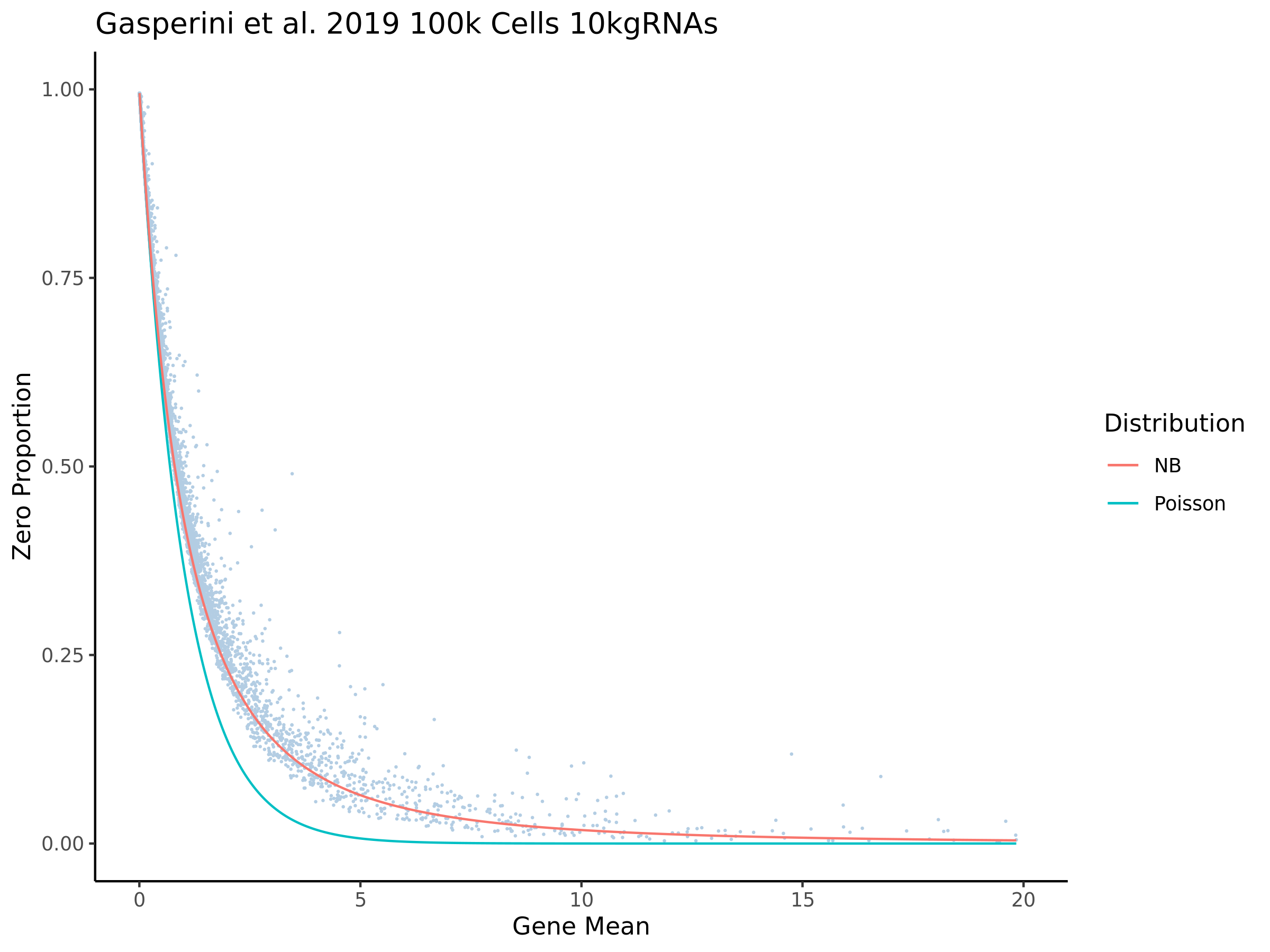
50k Cells (~25%) 10kgRNAs


All Cells 20kgRNAs


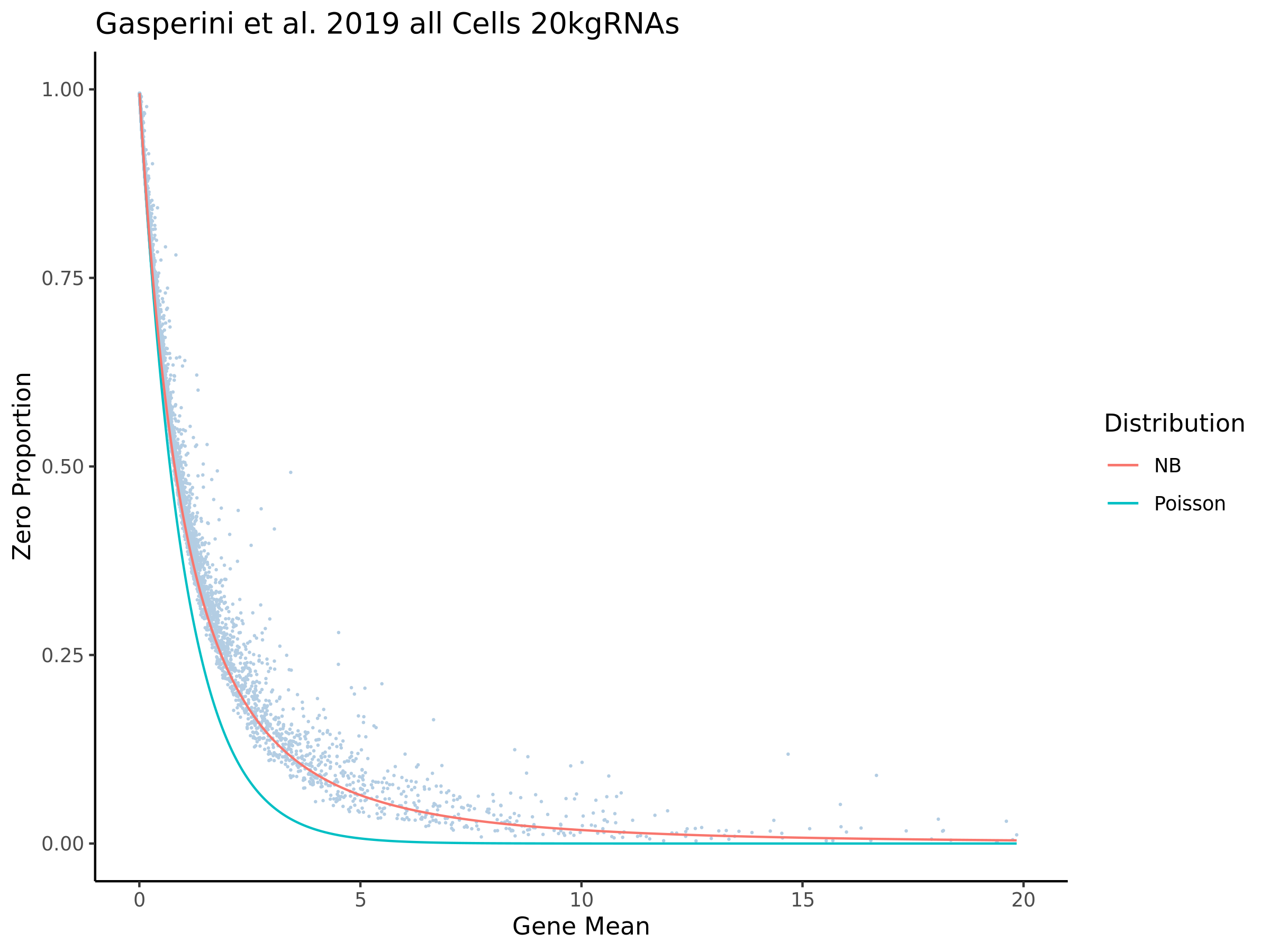
All Cells 30kgRNAs

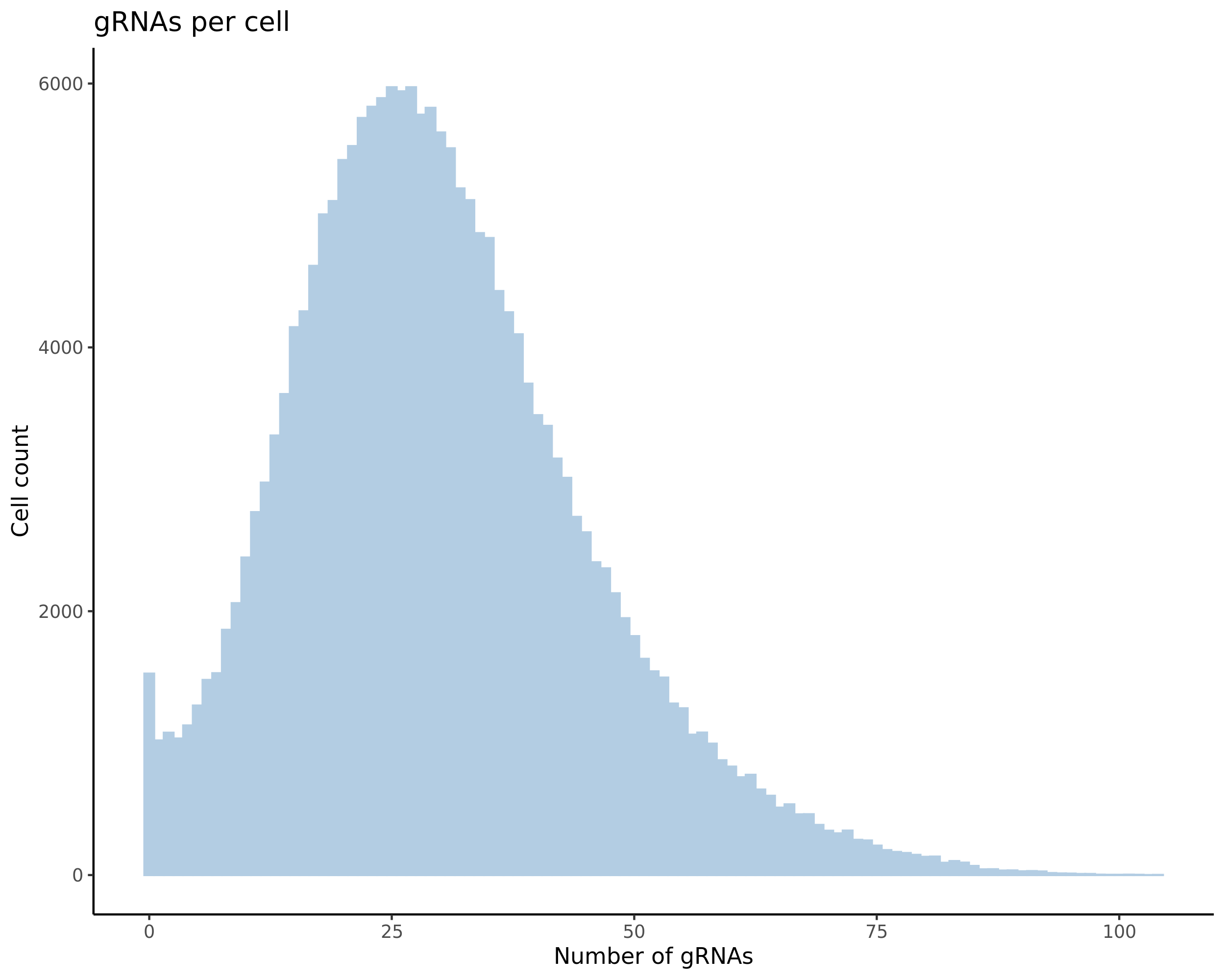

All Cells, MOI 20, 10kgRNAs


All Cells, MOI 10, 10kgRNAs

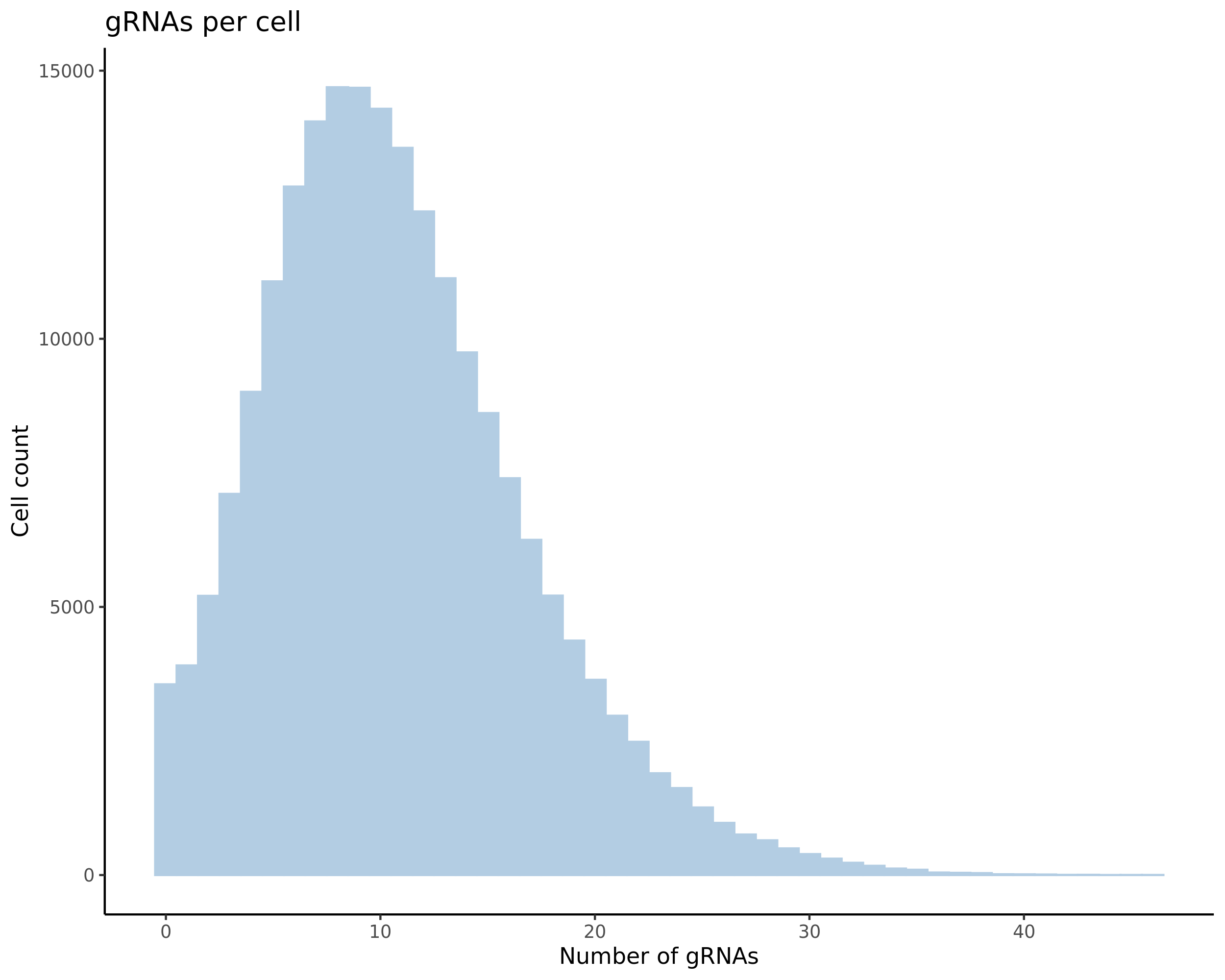

All Cells, MOI 5, 10kgRNAs

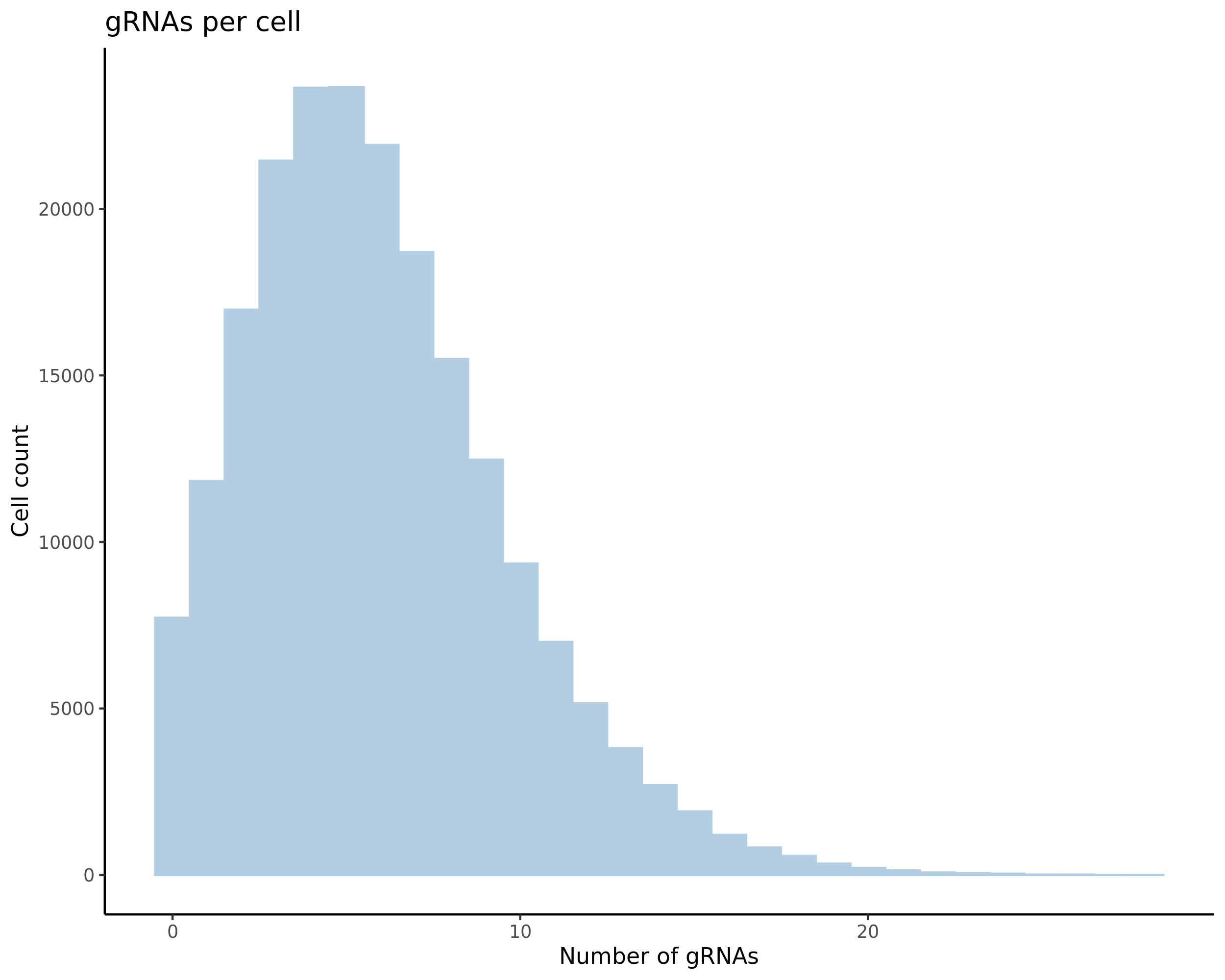

1/24/2022
Initial SCEPTRE Gasperini 2019 QC Results (TSS / NTC, cis)
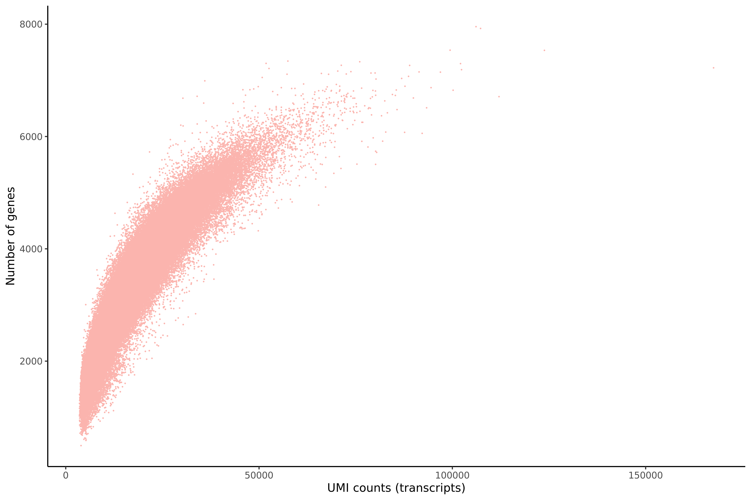
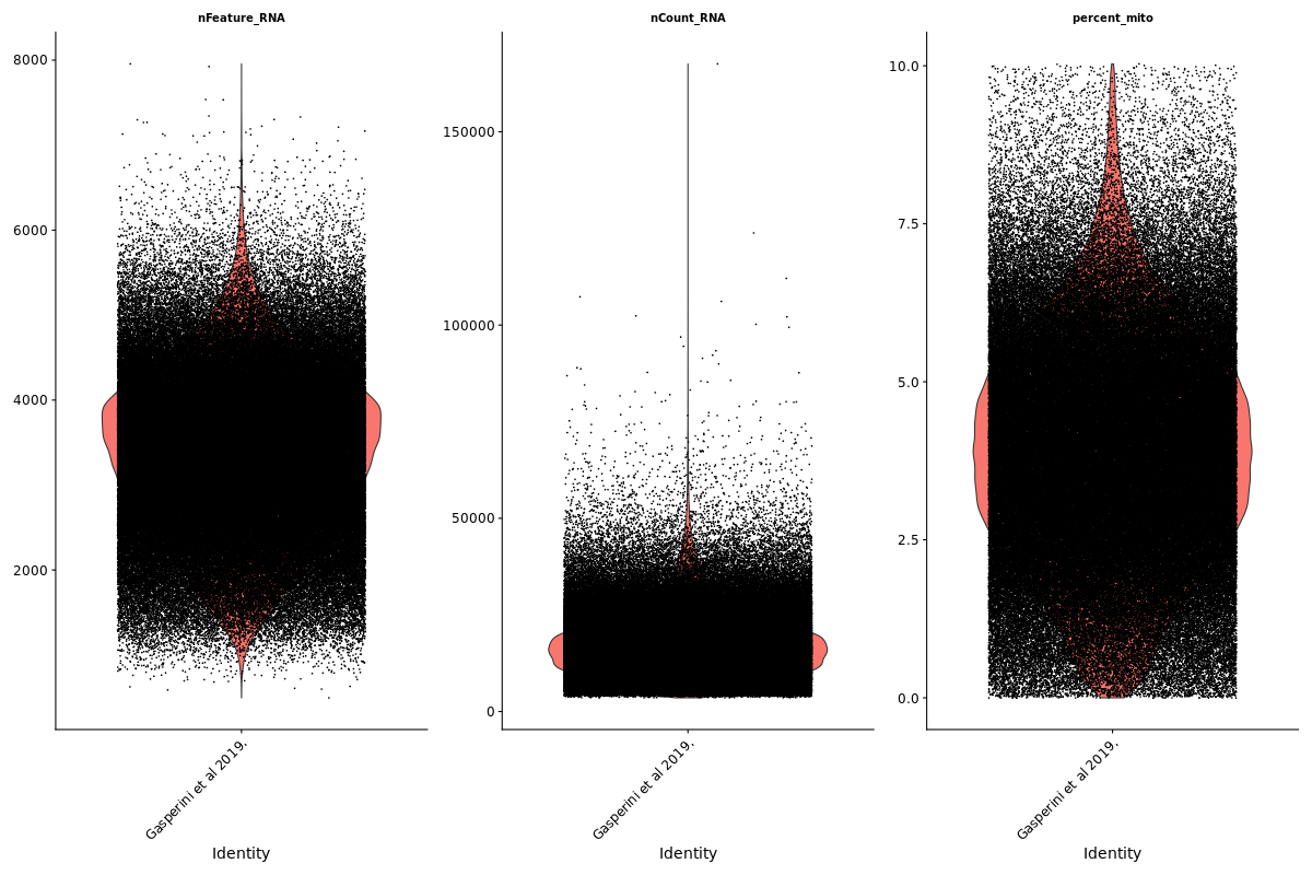
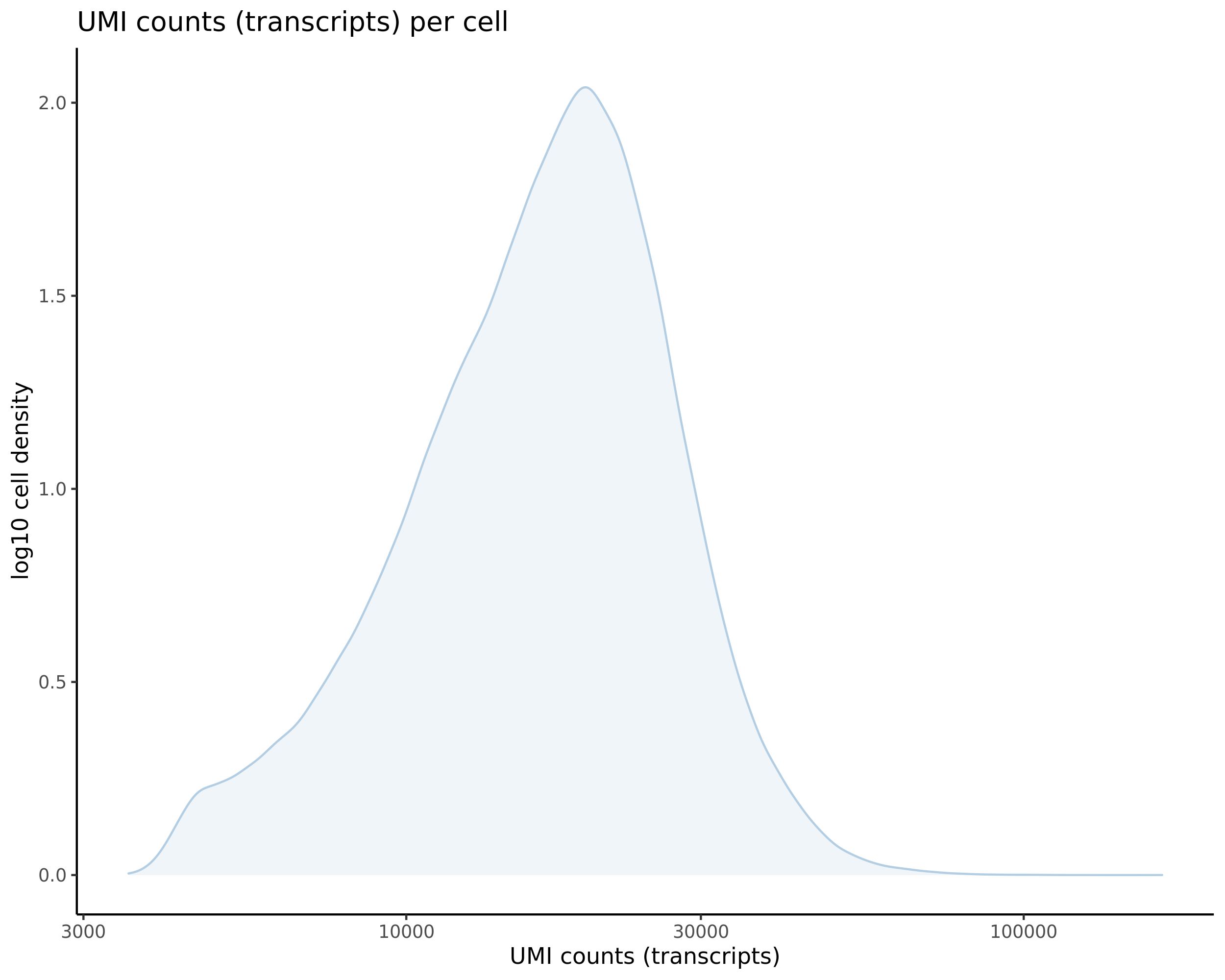
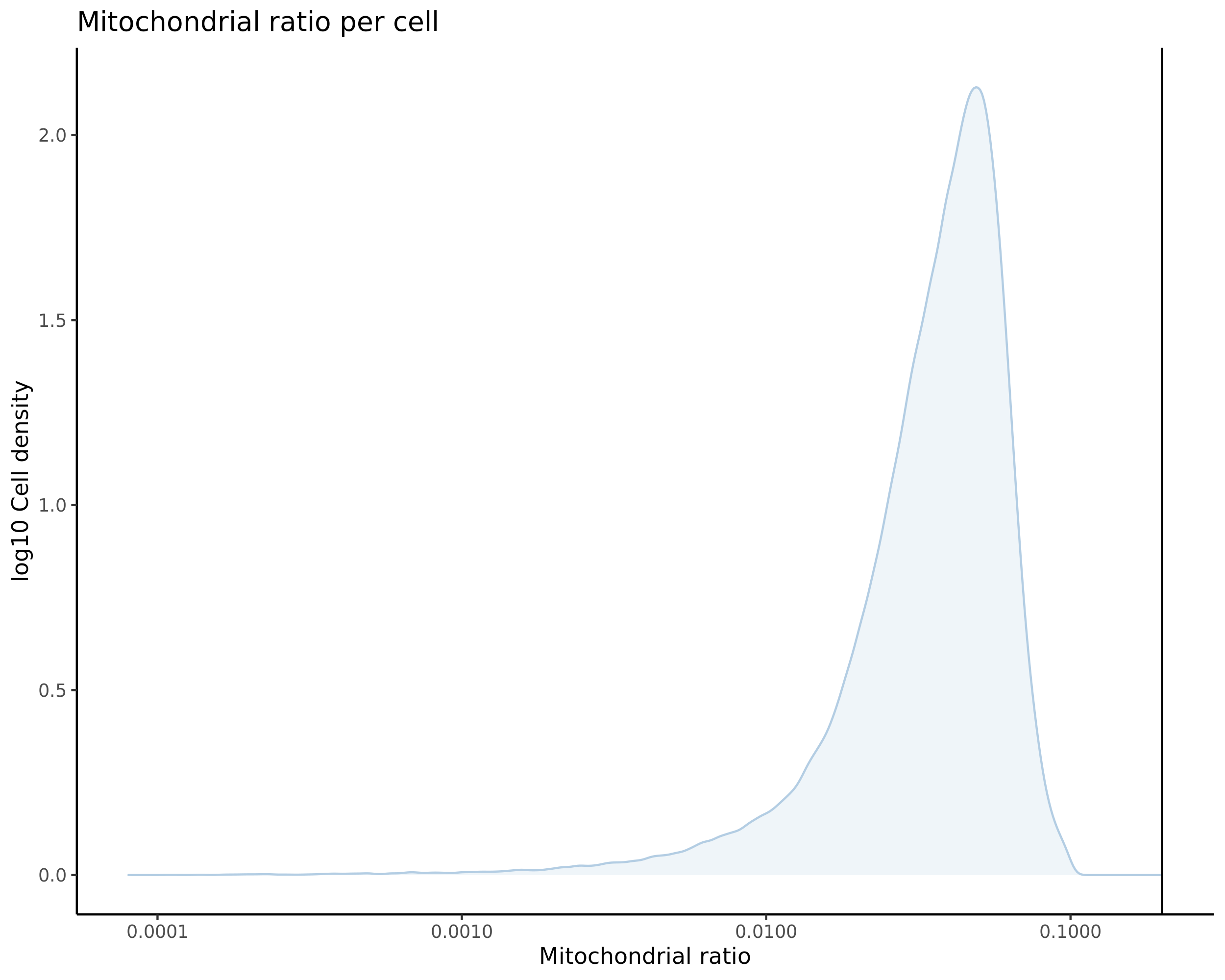

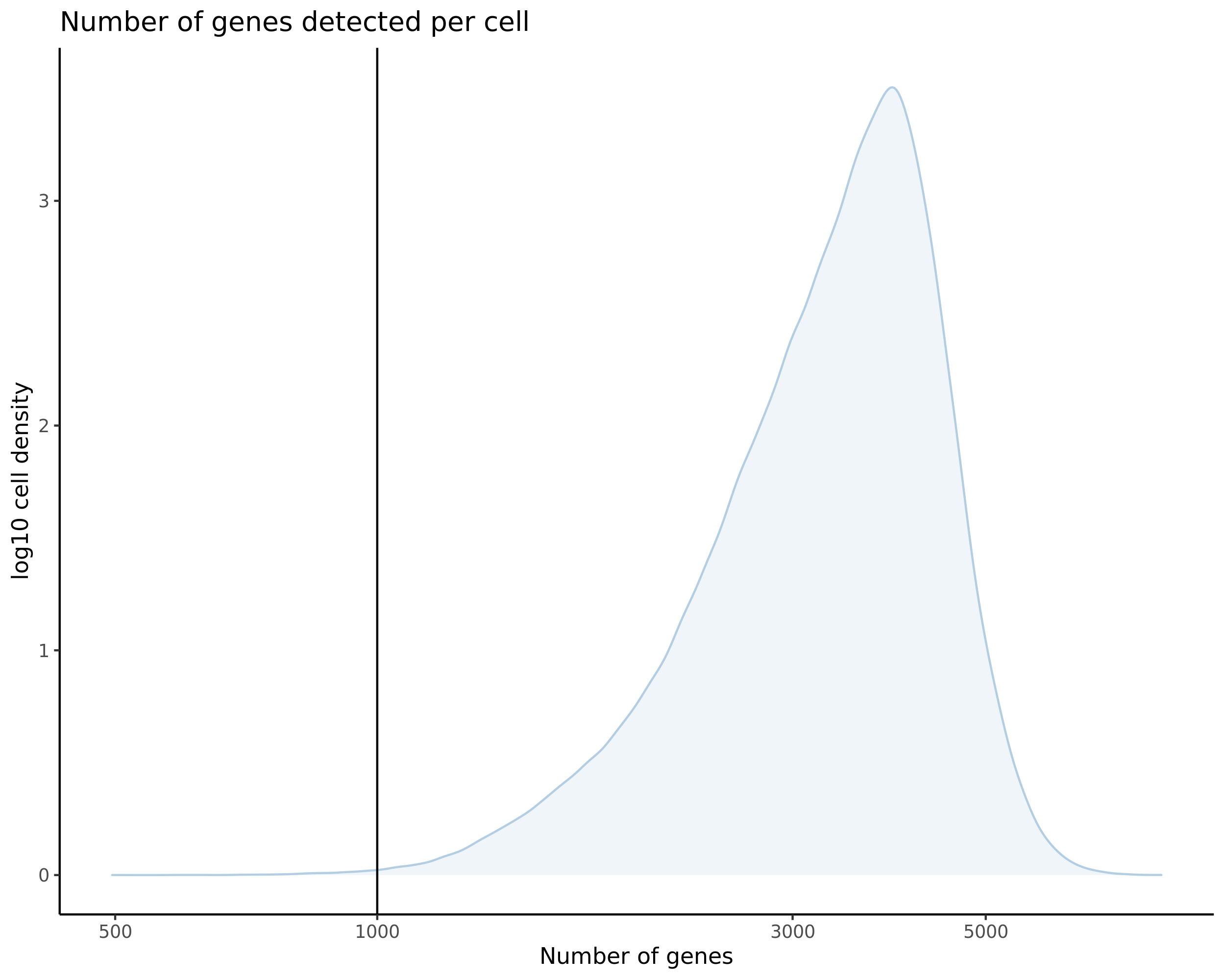
1/19/2022
Notes for SCEPTRE
Plan:
1. Download 3 datasets: Gasperini 2019, Datlinger 2017, and Morris 2021
2. Convert SCEPTRE into snakemake pipeline (preprocess to ondisc + sceptre analysis)
3. Replicate findings on trans-regulation
Current Steps:
1. Process Gasperini et al 2019 data for SCEPTRE
2. Run SCEPTRE to test gRNA-to-gene pairs in cis
3. Generate qqplot analogous to Figure 2.C in Morris 2021 bioxiv paper